Chapter 11 Probability

11.1 Objectives

The objectives of this chapter are to

• Understand the meanings, uses and ways of arriving at, numerical values for probabilities.

• Appreciate the context for a probability, and that context (the conditioning, the information relied on) matters.

• See the basic rules for calculating probabilities in a few examples, but appreciate that calculating non-standard probabilities should be left to experts. In practice, most of our probability values come from some pDistribution function, and we will encounter some of the 'off the shelf' ones in the next chapter.

• Be warned against calculating the wrong probability.

• Beware of intuition, especially with 'after the fact' calculations for non-standard situations.

Probability

• Meaning

• Long Run Proportion
• Estimate of (Un)certainty

• Amount prepared to bet

• Use

• Communicate one's (un)certainty about the value of a parameter
• Describe the randomness of data

• Measure how far data are from some hypothesized model

• How Arrived At

• Subjectively
• Intuition, Informal calculation, consensus Empirically Experience (actuarial, ...)
• Pure Thought
• Elementary Statistical Principles; if necessary, by breaking complex outcomes into simpler ones

• Advanced Statistical Theory, e.g.. Gauss' Law of Errors

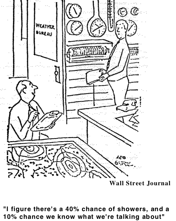
Figure 11.1: In this older cartoon, these experts qualify their probability statement.

What is the probability of/that ? ...

Death | Taxes | Rain tomorrow | Cancer in your lifetime | Win lottery in single try | Win lottery twice | Get back 11/20 pilot questionnaires | If treat 14 patients, get 0 successes | [Duplicate Birthdays(http://www.medicine.mcgill.ca/epidemiology/hanley/c323/excel/birthdays_607.pdf) | Canada will use $US before the year 2030 | another new/different pandemic by 2030 | OJ Simpson murdered his wife | DNA from a random (innocent) person would match blood found at crime scene

Often, we work in other scales that spread out the probability scale. The odds scale runs from 0 to in finity, while the logit and probit scales -- important for regression modeling -- span the entire real line, from minus infinity to infinity. You will need to become confortable with these wider scales.

11.2 Probability Scales

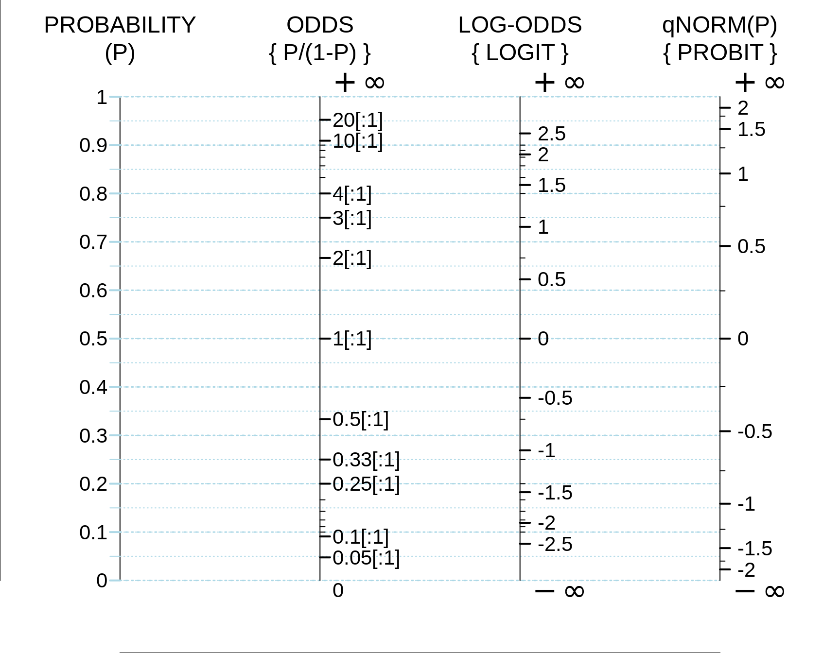
Figure 11.2: The probability scale, along with 3 equivalent scales derived from it. The probit scale transforms P into a Z score: thus P = 0.025 becomes Z = -1.96, and P = 0.975 becomes Z = +1.96; to reverse direction, if Z = qnorm(P), then P = pnorm(Z). To convert a LOGIT back to an odds, ODDS = anti-log(LOGIT) = exp(LOGIT), and to convert an odds back to a probability, P = ODDS/(1+ODDS).

• 50 year old has colon ca • 50 year old with +ve haemoccult test has colon ca • child is Group A Strep B positive • 8 yr old with fever & v. inflamed nodes is Gp A Strep B positive • There is life on Mars

References • WMS5, Chapter 2 • Moore & McCabe Chapter 4 •Colton, Ch 3 • Freedman et al. Chapters 13,14,15 •Armitage and Berry, Ch 2 • Kong A, Barnett O, Mosteller F, and Youtz C. "How Medical Professionals Evaluate Expressions of Probability" NEJM 315: 740-744, 1986 • Death and Taxes • Rain tomorrow • Cancer in your lifetime • Win lottery in single try • Win lottery twice • Get back 11/20 pilot questionnaires • Treat 14 patients get 0 successes • Duplicate Birthdays • Canada will use $US before the year 2010

11.3 Basic rules for probability calculations

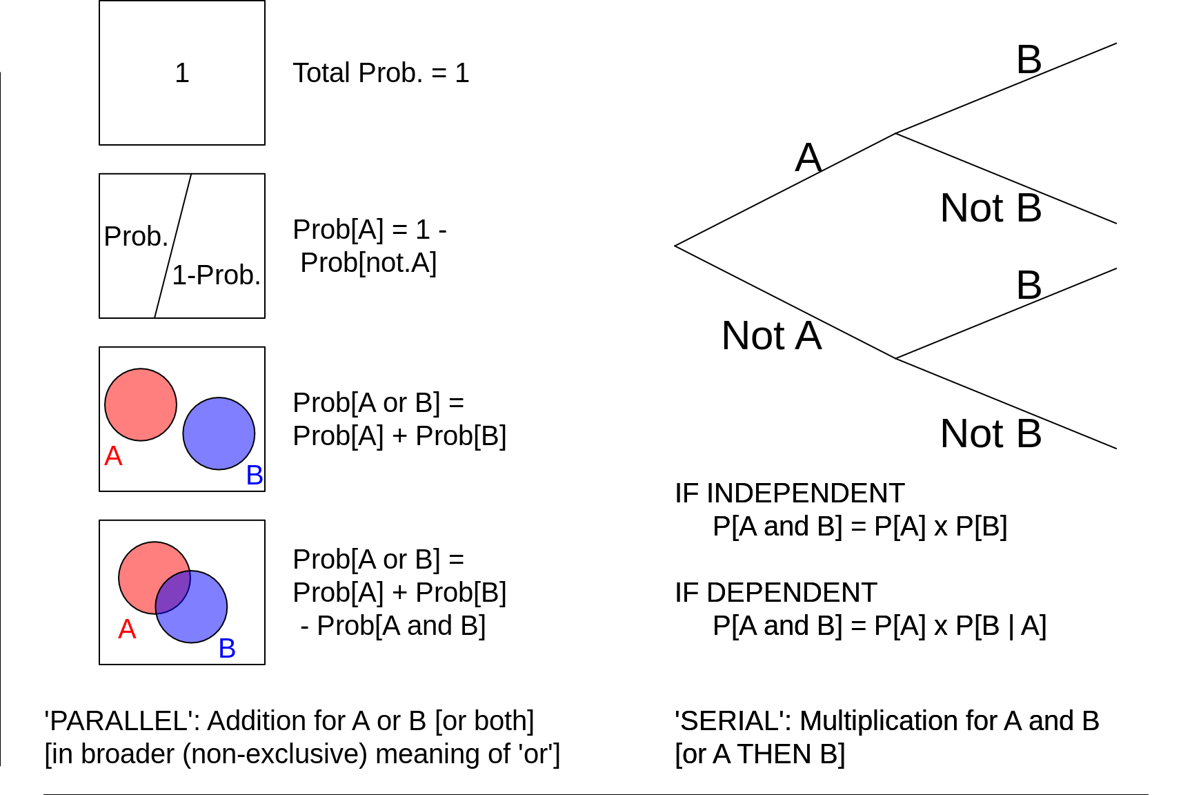
Figure 11.3: Basic Probablity Axioms and Rules. 'B | A' means 'B GIVEN A' or 'B CONDITIONAL ON A'.

11.4 Conditional probabilities, and (in)dependence

It is surprising how few textbooks use 'trees' (such as shown above) to explain conditional probabilities. Probability trees make it easy to see the direction in which one is preceeding, or looking, where simply (and often arbitrarily chosen) algebraic symbols like A and B can not; trees make it easier to distinguish 'forward' from 'reverse' probabilities. Tip: try to order letters so it is \(A\rightarrow B\), rather than \(B\rightarrow A.\)

Trees show that -- no matter whether the events are independent or dependent -- the probability of a particular sequence is always a fraction of a fraction of a fraction ... . Moreover we start with the full probability of 1 at the single entry point on the extreme left, so we need at the right hand side to account for all of this (i.e., the same ‘total’) probability. Just like the law of the conservation of mass, there is also a law on the conservation of probability; it cannot be lost or destroyed along the way.

This first example highlights the difference between independent events (left) and non-independent events (right).

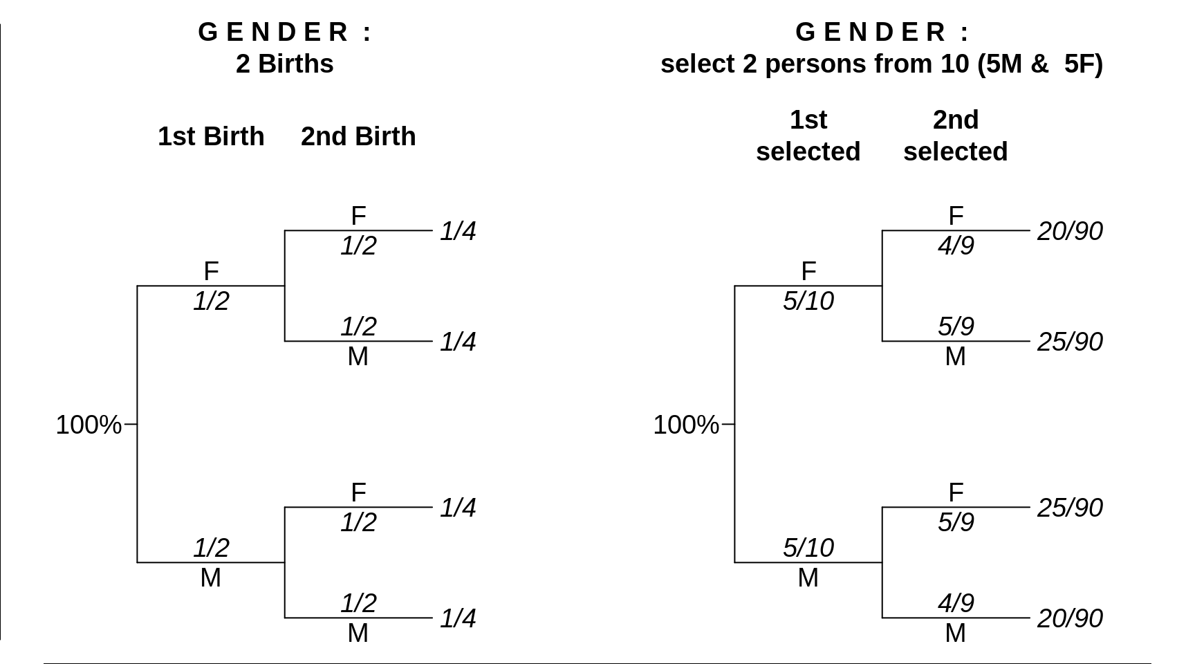
Figure 11.4: Gender Distribution in a sample of size \(n\)=2. LEFT: 2 independent Births; RIGHT: Randomly sampling 2 persons from 10 persons (5M 5F), without replacenent. In both examples, the terminal probabilities are obtained by multiplication. In the second example, the second probability depends on the outcome of the first selection.

With independence, one doesn’t have to look over one’s shoulder to the previous event to know which probability to use for the second portion of the product. In the example on the gender composition of 2 independent births, when one comes to the second component (birth) in the probability product, Prob(2nd birth is a male) is the same whether one has got to there via the 'upper' path, or the 'lower' one. 'Contitioning on' or 'knowing the result of' the first event does not alter the second probability.

With non-dependence, one does have to look at where one has come from. In the example on the gender composition of a sample of 2 persons sampled (without replacement) from a pool of 5 males and 5 females, the Prob(2nd person selected is a male) is differs depending on which path you have already taken.

The multiplication rules also apply to pairs of events that are not strictly serial in nature: the pairs can be assembled in other ways, such as in this second example.

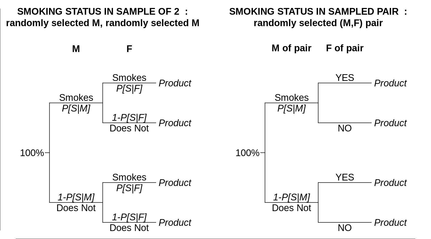
Figure 11.5: Another example of the difference between 'independent' and 'related' results. At issue is the composition of a make-female pair with respect to the number of sampled persons (out of \(n\) = 2) that smoke (0, 1, or 2). Left: the pair are formed at random, the Male selected randomly from all adult males, and the Female selected randomly from all adult females. Prob that F smokes is not realted to whether M does or does not. Right: a (related) M:F couple is selected from among all M:F couples, 'F, M+' denotes a Female whose M partner does smoke, and 'F, M-' denotes a Female whose M partner does not. These probabilities that these 2 types of Females smoke will differ from each other.

11.5 Changing the Conditioning: the direction matters

Example: Medical Diagnostic Tests

The left side of this next panel is an example where, when evaluating the performance of a new diagnostic test, we test selected numbers of persons known to have and not have the medical condition in question. To get reliable data on both the detection rate (or 'sensitivity', here assumed to be 90%), and the false positive rate (here 1%, making the 'specificity' 99%), we might (artificially) test roughly equal numbers of persons with and without the condition (here 40% and 60% of the total tested, making the 'prevalence' 40%). The right hand side reverses the process, so that it mimics clinical practice, where the test result is known, but the presence/absence of the condition is not. When the test result is positive, say, the question then, naturally, is the probability that the patient with the positive result has the condition of concern. If the prevalence were truly 40%, then we would have the numbers shown in the right hand panel. Clearly, in this setting, \[Prob[Disease \ is \ present \ | \ Test \ is \ Positive] \ne Prob[Test is Positive | Disease is present]\]

Figure 11.6: A first example of two very different sets of probabilities: LEFT The probabilities that a potential diagnostic test would be positive in persons who, respectively, do and do not have the medical condition of concern. RIGHT The probabilities that a medical condition of concern is present in persons whose diagnostic test is, respectively, positive and negative. It is assumed that the overall prevalence of the condition is 40%, just like in the population mix (left) it was evaluated on. Prob[Test is positive given that the Condition is Present] = 80%, but Prob[Condition is Present given that the Test is positive] is 87%.

In the following Figure, the detection rate and false positive rates are as before, but the prevalence of the condition being tested for is now only half as high, ie., 12.5%.

Figure 11.7: A second example of two differing different sets of probabilities: the detection rate and false positive rates are as before, but the prevalence of the condition being tested for is now only half as high. Prob[Test is positive given that the Condition is Present] = 80%, but Prob[Condition is Present given that the Test is positive] is 74%.

The 74% is called the 'positive predictive value' of the (positive) test. Sometimes the 74% is referred to as post-test (or more accurately the post-positive-test) probability.

The positive predictive value is lower still if the prevalence of the condition being tested for is lower again.

Example: The Etiologic Study

This 'hockey-epidemiology' example is based on data from 51 goals allowed by Canadiens goalie Patrick Roy in NHL games palyed again the Boston Bruins, and on the headline of the La Presse article: 'Pour battre Roy, mieux lancer bas' [to beat Roy, it's better to shoot low]

Since we don't have full data, the left side of this next panel is theoretical, and uses symbols for the unknown probabilities. We would like to know the difference between Prob[Goal | Shoot Low] and Prob[Goal | Shoot Low], but if worst comes to the worst, we would settle for the ratio Prob[Goal | Shoot Low] : Prob[Goal | Shoot High],

The RIGHT hand side illustrates the modern conception of THE etiologic study, using a case series (in this example, the series is 51 goals) and a base series (100 random shots selected from the videotapes of the games in question: it would take too long to examine and classify all 100% of the shots as low/high).

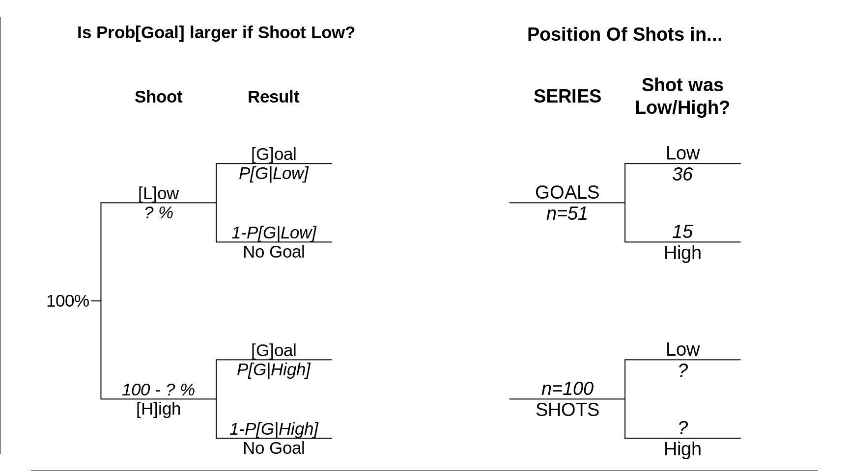
Figure 11.8: A first example of the difference between two very different sets of probabilities. The LEFT panel allows one to estimate (in the 2nd column) the exposure-specific rates (incidence densities) of developing lung cancer, The RIGHT panel begins from a case series of size n, and couples it with a base (denominator) series K times that size that estimates the distribution of smoking histories in (from a representative sample of) the base -- the experience from which the cases arose. The exposure-specific numerators (numbers of cases) and estimated exposure-specific relative-denominators allow for the estimation of an incidence density ratio.

The difference between 'forward' and 'reverse' probabilities distinguishes frequentist p-values (probabilities) from Bayesian posterior probabilities.

\[Probability[ data \ | \ Hypothesis ] \neq Probability[ Hypothesis \ | \ data ]\]

or, if you prefer something that rhymes,

\[Probability[ \ data \ | \ theta ] \neq Probability[ \ theta \ | \ data ].\]

Example: The Prosecutor's Fallacy

Here, in the context of criminal trials involving DNA evidence, are two striking -- and worrysome -- examples of misunderstandings about them. This misunderstanding is often referred to as the 'Prosecutor's Fallacy'.

In the 1995 OJ Simpson trial - the subject of this recent tv series -- the (very very small) probability that the blood of a randomly-selected innocent person would match that found at the crime scene was mistaken as (confused with) the probability that the person accused of murder was innocent. It is worth repeating an excerpt from JH's bios601 notes, just cited.

In this case the statistician Peter Donnelly opened a new area of debate. He remarked that
.
forensic evidence answers the question: What is the probability that the defendant’s DNA profile matches that of the crime sample, assuming that the defendant is innocent?
.
while the jury must try to answer the question
.
What is the probability that the defendant is innocent, [in the light of ALL of the OTHER EVIDENCE and] assuming that the DNA profiles of the defendant and the crime sample match?

The OJ Simpson case also features a well-known Harvard law professor Alan Dershowitz-- who was in the news again in the Trump impeachment case -- whose insunuations and misuse of probabilites spurred the renowned and respected statistician IJ Good (who and worked with Alan Turing) to write this article in the journal Nature. It begins:

SIR - Alan M. Dershowitz, who advises the defence lawyers in the 0. J. Simpson trial, stated on US television in early March that only about a tenth of 1% of batterers actually murder their wives. His statement, though presumably true, is highly misleading for the woman in the street. A probability of greater relevance for legal purposes would be based on the knowledge that the woman was both battered by her husband and also murdered by somebody. An approximate estimate of this probability will now be made, based on Dershowitz's statement.

Some statistical articles, having to do with lie detection tests, have also mixed up the probability of innocence given data with the (much easier to calculate) probability of data given innocence.

Naive Measures of diagnostic/prognostic accuracy

Many claims of high accuracy of diagnostic or screening tests rely on artificially-high rates of the target condition, and/or combine the 'sensitivity' and 'specificity' performance measures into one number.

11.6 Summary Slides

• Probablities can be viewed as long-run frequencies, or as degrees of belief.

• We often map probabilities into, and work with, other scales.

• The 'calculus' of probabilities relies on additions and subtractions, and multiplications.

• There is always a context for a probability.

• Trees can help to keep things (and directions!) straight.

• When things are more complex, simulations can help.

• It is easy to confuse contexts, and to calculate the wrong probability.

• \[Probability[ data \ | \ Hypothesis ] \neq Probability[ Hypothesis \ | \ data ]\]

• \[Probability[ \ data \ | \ theta ] \neq Probability[ \ theta \ | \ data ].\]

• Don't fall into the 'prosecutor's fallacy' trap, and mistake a p-value for the probability that the (null) hypothesis is true.

• Be suspicious of small (extreme) probabilities: they may well have been incorrectly calculated, or not all that revevant.

11.7 Exercises:

1. Convert the proportion of male births to a sex ratio, and to the log of the sex ratio. If, because of natural year to year variations, the proportion varies from 0.49 to 0.53, what does the ratio vary from? the log of the ratio? What if proportion were 3/4. scales SDs See John Arbuthnot's data.

2. In a recent report, the focus was on the proportion of persons who would detect added (spiked) alcohol in a drink. The authors fitted a logistic S curve, and arrived at the equation \[ logit[proportion \ if \ X \ = \ x] \ = \ x.x - y.y \ Dose.\]. From this, calculate the fitted proportion if X = zzz.
   The authors alos fitted a probit-based S curve, and arrived at the equation \[ probit[proportion \ if \ X \ = \ x] \ = \ w.w - q.q \ Dose.\]. From this, calculate the fitted proportion if X = zzz.

3. In an older report, the focus was on the proportion of persons who had reached menarche by a given age. The authors fitted a logistic S curve, and arrived at the equation \[ logit[proportion \ if \ X \ = \ x] \ = \ x.x - y.y \ Age.\]. From this, calculate the fitted proportion if X = zzz.
   The authors also fitted a probit-based S curve, and arrived at the equation \[ probit[proportion \ if \ X \ = \ x] \ = \ w.w - q.q \ Age.\]. From this, calculate the fitted proportion if X = zzz.

4. Suppose you measure the heights of a randomly chosen adult male and a randomly chosen adult female, and record where each one is relative to the (a) Q\(_{25}\) (b) Q\(_{50}\) (median) and (c) Q\(_{75}\) value of their same-sex peers, and mark the result on a 3 x 3 grid (like the grid Galton used). For each of the 9 cells, what is the probability that they will be that cell?

5. "Clustering" of Cardiovascular Risk Factors ?
   A Santé Quebec survey found the prevalence of 4 heart disease risk factors in a certain age-sex group to be: smoking: 32%; family history: 32%; SBP>155mmHg: 12%; diabetes: 5%. If risk factors are distributed independently of each other, what is the proportion of the age-sex group with (a) 4 risk factors (b) 0 risk factors (c) 1 or more risk factors?. A tree diagram may help.

6. Suppose that the probability that HIV will be passed from an infected person to an uninfected person during a single sexual contact is 0.01. Suppose that there are 50 such contacts. Show how to calculate (or obtain via software) the probability that HIV will be passed on in at least one of the 50 contacts.

7. Refer to a (current) lifetable calculated from (made with) with recent mortality data, For example, Table 3.9 in this Quebec report.

• Why is the average (expected) age at death of 20 years old males 81.2 years while that for 30 years olds is 81.6? and 84.8 and 84.9 for females?
• Why did William Farr, in the Fifth Report of the Registrar General 1843 say that

a strong case may no doubt be made out on behalf of those young, but early-dying Cornets, Curates, and Juvenile Barristers, whose mean age at death was under 30! It would be almost necessary to make them Generals, Bishops, and Judges — for the sake of their health. [The answer is in the page before]

7. continued

• Why did the International Journal of Epidemiology report of these Danish investigators generate the headline 'Soldyrkere lever meget længere' -- 'Sun worshipers live much longer' and the subtitle: 'New research among 4.4 million Danes shows that sun worshipers on average live six years longer?

8. An auto insurance company notes whether drivers under 21 years old have had a driver’s education course. Some 40% of its policyholders under 21 have had a driver's education course and 5% of this subset have an accident in a one-year period. Of those under 21 who have not had a driver’s education course, 10% have an accident within a one-year period.
   A 20-year-old takes out a policy with this company and within one year has an accident. What is the probability that the person did not have a driver's education course? [a probability tree may help] 607 midtern 2001

9. Twins: [Real story from a real statistician]
   Depict Efron’s calculations using a probability tree. Here is his story"

Here is a real-life example I used to illustrate Bayesian virtues to the physicists. A physicist friend of mine and her husband found out, thanks to the miracle of sonograms, that they were going to have twin boys. One day at breakfast in the student union she suddenly asked me what was the probability that the twins would be identical rather than fraternal. This seemed like a tough question, especially at breakfast. Stalling for time, I asked if the doctor had given her any more information. 'Yes', she said, 'he told me that the proportion of identical twins was one third'. This is the population proportion of course, and my friend wanted to know the probability that her twins would be identical.
Bayes would have lived in vain if I didn’t answer my friend using Bayes' rule. According to the doctor the prior odds ratio of identical to nonidentical is one-third to two-thirds, or one half. Because identical twins are always the same sex but fraternal twins are random, the likelihood ratio for seeing 'both boys' in the sonogram is a factor of two in favor of Identical. Bayes' rule says to multiply the prior odds by the likelihood ratio to get the current odds: in this case 1/2 times 2 equals 1; in other words, equal odds on identical or nonidentical given the sonogram results. So I told my friend that her odds were 50-50 (wishing the answer had come out something else, like 63-37, to make me seem more clever.) Incidentally, the twins are a couple of years old now, and 'couldn’t be more non-identical' according to their mom. [Bradley Efron]

10. Screening for HIV: Can we afford the false positive rate?

• Represent the information they use in their Meaning of Postive Tests section (starting on page 239, second column) as a tree.
• Then present the same information in a different tree, with data [test result] on left, and hypothesis on the right (rather than the conventional \(\theta \rightarrow\) data' direction)
  .

11. The Economist article Problems with scientific research: HOW SCIENCE GOES WRONG

has a very nice graphical explanation of why some many studies get it wrong, and cannot be reproduced -- the topic of the Reproducibility Project in Psychology referred to on same page.

One reason is that even if all studies were published, regardless of whether the p-value was less than 0.05 (a common screening/filtering criterion) or greater than 0.05, of all the hypotheses tested, only a small percentage of the hypotheses are 'true'. Thus many or most of the 'positive' tests (published results) will be false positives. It is just like when using mammography to screen for breast cancer: in maybe 4 of every 5 women referred for biopsy, the biopsy will come back negative.

• Represent the information in their Figure as a tree. Then present the same information in a different tree, with data on left, and hypothesis on the right (rather than the conventional \(\theta \rightarrow\) data' direction) -- as JH has done in a few instances above.

• What percentage of positive tests would be correct/not if, instead, 1 in 2 of the hypotheses interesting enough to test were true?

• Come up with a general formula for what in medicine is called the 'positive predictive value' of a positive medical test.

• Try to simplify it so that the characteristics of the test(\(\alpha \ and \ \beta\) are isolated in one factor, and the testing \underline{context (the 1 in 10 or 1 in 2, etc.) is in another. Hint: use odds rather than probabilities, so that you are addressing the ratio of true positives to false positives, and the ratio of true hypothesis to false hypotheses. And use the Likelihood Ratio

• On the same Resources web page is another (but longer) attempt to explain these concepts graphically to left brain and right brain doctors. JH was impressed with this, and wanted to share it with the Court for Arbitration in Sport, when explaining the interpretation of positive doping tests. But he found that the 'teaser' sentence immediately following the title, ''Can you explain why a test with 95% sensitivity might identify only 1% of affected people in the general population?'' is misleading, and so he make his own diagram (available on request). Exercise: Revise this misleading phrase. and see this shiny app.

8. Wald : CF screening

9. OJ p-value

10. Adult soccer ball.. wrong probability

11. Vietnam deaths

12. NHL birthdays

Medical School admission rates, by gender.

Vietnam war deaths, by month of birth

NHL success, by month of birth

John Snow, cholera deaths South London, by source of drinking water