Chapter 18 Computing: Session No. 4
18.1 Objectives
The 'computing' objective is to learn how to use R to simulate variation by (Monte Carlo) simulation. Tasks and R Functions/structures used include
Read a file in table format and creates a data frame from it, with cases corresponding to lines and variables to fields in the file"
read.table( )Compactly display the internal
structure of an R object, e.g. the abbreviated contents of (possibly nested) lists:str( )repeating a procedure for subsets of a dataframe:
by( )loops using
for. See here.rescaling a vector
vso that it sums to 1:v = v / sum(v)adding elements of a vector or (say) a product of 2 vectors, or a square of a vector: `sum( )
compute the mean and standard deviation of the numbers in a vector:
mean()andsd( )computing the mean and SD of a (population) frequency distribution from first principles using the scaled frequencies as probabilities:
sum(values*probabilities)extracting the first or last parts of a vector, matrix, table, or data frame:
head( )andtail( )removing duplicate elements/rows from a vector, data frame or array:
uniqueplotting:
plot( )adding one or more straight lines through the current plot:
abline( )joining multiple (x,y) points with line segments:
lines( )Splitting data into subsets, computing summary statistics for each, and returning the result in a convenient form:
aggregatesampling from a set of values:
sample( )summing the values in a vector:
sum( )applying a function to each of the rows or columns of a matrix, or to some slices of higher-dimensional array:
apply( )computing the mean, variance and sd of a vector:
mean( ),var( ),sd( )defining a (homemade) function to 'automate' a procedure
functiontabulating the values in a vector, or crosstabulating the values in 2 or more vectors:
table( )
The 'statistical' objective of this exercise is to learn-by-seeing some of the laws that describe/quantify the variation (variance, SD) of the sum, and more importantly, the difference of 2 random variables. The laws are the same no matter whether the difference is in some characteristic of 2 randomly selected individuals or in some statistic (an aggregate of individual values). Since we don't get to see the individuals -- or collections of individuals -- that were nor selected, the laws are based on the theory of mathematical statistics, and thus not easy to visualize/imagine. So, we will use simulations (virtual thought experiments) to help us motivate and remember the laws, and to bring out the possibly-surprising 'reasons why' they take the form they do.
The take-home message is that if the two random quantities involved in the difference are statistically independent of each other, the possible variations in the difference are larger than the ones in each of the two components, and that Variances Add; SDs don't. The variance of a sum or difference is equal to the sum of the (variances of the) parts
In the case of all things which have several parts and in which the totality is not, as it were, a mere heap, but the whole is something besides the parts, there is a cause; for even in bodies contact is the cause of unity in some cases, and in others viscosity or some other such quality. Aristotle’s Metaphysics. Book VIII, 1045a.8–10 1908 translation by W. D. Ross:
The whole is greater than the part. Euclid, Elements, Book I, Common Notion (Euclid is expressing how a whole can be split into parts, and any one of those parts, compared to the whole, is less than the whole. And using the Segment Addition Postulate – If point P is between points A and B, then AP + PB = AB. Ipso facto, the sum of parts equal the whole.
that the whole is not the same as the sum of its parts are useful in meeting the type just described; for a man who defines in this way seems to assert that the parts are the same as the whole. The arguments are particularly appropriate in cases where the process of putting the parts together is obvious, as in a house and other things of that sort: for there, clearly, you may have the parts and yet not have the whole, so that parts and whole cannot be the same.” Aristotle. Book VI. (all of the above are from this URl.
Likewise, the SD of a sum or difference is less than the sum of the (SDs of the) parts
Although the theoretical chapter does not address the laws for sums or differences of non-independent random variables, the simulations bring out the fact that the variance of the sum/difference could be bigger or smaller than the variances of the parts: it all depends on how the components are linked.
18.2 Exercises
First, before we get to differences, an example of the sampling variability of sums and means.
The sex-specific panels below shows examples of the sums of the lengths of 10 baby names, placed side by side. (each row includes 9 blank spaces, so that doesn't change the variability: it just shifts all the sums by 9.) The fact that they are not randomly ordered, bur rather ordered by popularity, doesn't matter that much, since -- as the subsequent graph shows -- popularity is not strongly related to the length of the name. Had we randomly ordered them, we would still see the 'jagged' line endings and the same anount of variation. (Ignore for now the last column, which shows a type of sampling that is to be discouraged, or that, if used, needs post-hoc adjustment of the results).
18.2.1 Ages of UK cars
Refer to the exercise, and the dataset, in the first computing session.
Using the year-of-manufacture frequency distribution you derived back then, calculate the mean year, and thus the mean age.
From first principles, i.e., using devaitions from the mean year, calculate the variance -- and thus the SD -- of the distribution.
Without actually converting every year-of-manufacture to an age, calculate the standard deviation of the ages.
Even though the frequency distribution is not symmetric, how could the SD (or an estimate of it) be of help if you had to estimate the mean age from just a random sample of registered cars.
18.2.2 Lengths of Babies' Names
The 500 most popular baby names, Quebec, 2013-1018
from="https://www.retraitequebec.gouv.qc.ca/en/services-en-ligne-outils/banque-de-prenoms/Pages/recherche_par_popularite.aspx?AnRefBp=2018&NbPre=0&ChAff=PPMP&NbPrePag=500"

ds = read.table(
"http://www.biostat.mcgill.ca/hanley/statbook/QuebecBabyNames2013to2018.txt",
as.is=TRUE)

str(ds)
## 'data.frame': 6000 obs. of 6 variables:
## $ Name : chr "LEA" "EMMA" "OLIVIA" "FLORENCE" ...
## $ Frequency: int 636 518 505 457 447 422 408 370 355 349 ...
## $ Length : int 3 4 6 8 5 3 7 8 5 7 ...
## $ Year : int 2013 2013 2013 2013 2013 2013 2013 2013 2013 2013 ...
## $ Gender : chr "F" "F" "F" "F" ...
## $ Rank : int 1 2 3 4 5 6 7 8 9 10 ...by(ds,list(g=ds$Gender,y=ds$Year),head,n=3)## g: F
## y: 2013
## Name Frequency Length Year Gender Rank
## 1 LEA 636 3 2013 F 1
## 2 EMMA 518 4 2013 F 2
## 3 OLIVIA 505 6 2013 F 3
## ------------------------------------------------------------
## g: M
## y: 2013
## Name Frequency Length Year Gender Rank
## 501 WILLIAM 848 7 2013 M 1
## 502 NATHAN 792 6 2013 M 2
## 503 SAMUEL 716 6 2013 M 3
## ------------------------------------------------------------
## g: F
## y: 2014
## Name Frequency Length Year Gender Rank
## 1001 EMMA 580 4 2014 F 1
## 1002 LEA 579 3 2014 F 2
## 1003 OLIVIA 520 6 2014 F 3
## ------------------------------------------------------------
## g: M
## y: 2014
## Name Frequency Length Year Gender Rank
## 1501 WILLIAM 787 7 2014 M 1
## 1502 THOMAS 742 6 2014 M 2
## 1503 FELIX 721 5 2014 M 3
## ------------------------------------------------------------
## g: F
## y: 2015
## Name Frequency Length Year Gender Rank
## 2001 EMMA 631 4 2015 F 1
## 2002 LEA 540 3 2015 F 2
## 2003 OLIVIA 482 6 2015 F 3
## ------------------------------------------------------------
## g: M
## y: 2015
## Name Frequency Length Year Gender Rank
## 2501 WILLIAM 767 7 2015 M 1
## 2502 THOMAS 762 6 2015 M 2
## 2503 JACOB 671 5 2015 M 3
## ------------------------------------------------------------
## g: F
## y: 2016
## Name Frequency Length Year Gender Rank
## 3001 EMMA 643 4 2016 F 1
## 3002 LEA 517 3 2016 F 2
## 3003 OLIVIA 516 6 2016 F 3
## ------------------------------------------------------------
## g: M
## y: 2016
## Name Frequency Length Year Gender Rank
## 3501 WILLIAM 798 7 2016 M 1
## 3502 THOMAS 701 6 2016 M 2
## 3503 LIAM 666 4 2016 M 3
## ------------------------------------------------------------
## g: F
## y: 2017
## Name Frequency Length Year Gender Rank
## 4001 EMMA 620 4 2017 F 1
## 4002 LEA 557 3 2017 F 2
## 4003 ALICE 519 5 2017 F 3
## ------------------------------------------------------------
## g: M
## y: 2017
## Name Frequency Length Year Gender Rank
## 4501 WILLIAM 714 7 2017 M 1
## 4502 LOGAN 675 5 2017 M 2
## 4503 LIAM 634 4 2017 M 3
## ------------------------------------------------------------
## g: F
## y: 2018
## Name Frequency Length Year Gender Rank
## 5001 EMMA 612 4 2018 F 1
## 5002 ALICE 525 5 2018 F 2
## 5003 OLIVIA 490 6 2018 F 3
## ------------------------------------------------------------
## g: M
## y: 2018
## Name Frequency Length Year Gender Rank
## 5501 WILLIAM 739 7 2018 M 1
## 5502 LOGAN 636 5 2018 M 2
## 5503 LIAM 629 4 2018 M 3
Figure 18.1: The closely spaced vertical lines show the frequency distributions of the popularity (ranks) of the 500 most popular names for babies born in Quebec in 2018. For example, more than 600 girls and more than 700 boys had the most popular name, while fewer than half this many babies had the 25th most popular name. Also shown are the names themselves, arranged row-wise, starting from the most popular (1. Emma 2. Alice, .. 1. William, 2. Logan, ...). For each row, the two values shown in plain type are the sum/mean of the lengths of the 10 names in the row. The last number, in italics, is the length of 1 name selected from the row, by 'sticking a pin' (indicated by the black ^ symbol), at random in one of the letters in the row, and selecting the name that the pin landed on. The values in bold at the foot of each column are the mean and SD of the values in the column.
par(mfrow=c(2,1),mar = c(5,5,0,0)) # splits graph into 2 x 1 grid

 for( g in unique(ds$Gender) ) {

  d = ds[ds$Gender == g,]

  COL=c("red","blue")[1 + (d$Gender=="M")]

  plot(d$Length,d$Rank, pch=19, col= COL, cex=0.25,
       ylab="Rank", xlab = "Number of Letters in Name",
       ylim=c(0,570) )
  abline(h=seq(0,500,50),col="lightblue")
  lines(aggregate(d$Rank,by=list(Length=d$Length),mean))
  Fr = aggregate(!is.na(d$Rank),by=list(Length=d$Length),sum)
  L = Fr$Length
  Fr = Fr$x
  text(min(L),550,"Cum. %",adj=c(0.5,-0.1),cex=0.75)
  for(i in 1:length(L) ) text(
         L[i], 510,
         toString( round( 100*cumsum(Fr)/3000) [i] ),
         adj = c(0.5,-0.1), cex=0.75 )
 }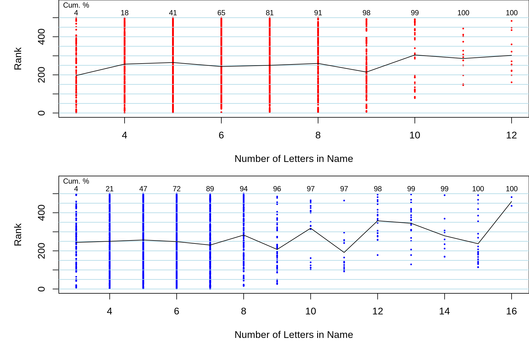
Figure 18.2: For girls (red) and boys (blue) separately, the mean ranks of names with a given length are plotted against the length. Each dot in a column is a name. The relative densities of the dots in a column indicates how common these name lengths are.
Exercise
Use the
LengthandFrequencycolumns in thedsdataframe (see above) to compute the (gender-specific) mean and SD of the lengths of the names of all of the Quebec babies born in 2018 having one of these names (For our purposes here, the few percent of babies whose names did not make it into the top 500 are excluded. If interested, they can be found at the link shown above.) Hint: you could rescale theFrequencyvector so that it sums to 1, and then simply use thesumof its product withLength. You can think of the rescaledFrequencyvector as probabilities.Rather than do these computations separately for each year, find a way to automate this. Hint: maybe put what you did to compute the mean and SD for one year into your own
functionand then use this function in abystatement. For example, if all you wanted was the number of babies each year, you could just use the inbuilt functionsum, and apply it to the frequencies in each year, using the statementby(ds$Frequency,ds$Year,sum).Compare your SD calculations agaist the SD[lengths of 500 names] shown at the bottom left of the red and blue panels of names, and if they are different, explain why they are.
Using the SD[lengths of 500 names] values shown, explain why the 2 SD's in bold to the right of them (at the feet of the two columns) are so much bigger or smaller. Do these 2 SDs in bold 'fit' with the laws we are learning about? Explain.
Use Monte Carlo simulations -- and the fact that you KNOW the gender-specific mean and SDs of the lengths of names -- to check out the theoretical formulae (laws) for the possible variation in the difference of two sample means. In other words, with \(y\) denoting the length of the name of a randomly selected baby, \(n\) the size of each sample, and \(\sigma\) denoting the unit standard deviation, and \(F\) and \(M\) denoting female and male, show -- to within Monte Carlo error -- that \[ Var[ \bar{y}_{F} - \bar{y}_{M} ] = \frac{\sigma^2_{F}}{n} + \frac{\sigma^2_{M}}{n}.\] Use '\(n\)'s of size 5, 25, 100, and 400. Use the
samplefunction with the rescaled frequencies as probabilities, andreplace = TRUE. To keep the computing simpler, limit yourself to one year. Here is some starter code. You need to modify it to extend the sample size to 400, add to thefunctioncode so that it includes samples of females, and computes the \(\bar{y_F} - \bar{y_M}\) fifference. (theresultsmatrix has 3 columns, only 1 of which gets filled under the present code.) You should try a small value ofN.SIMSfirst, to be sure everyting is working, and then make it large so that you approach the 'expected' values. Note: this code uses loops, which are slower, to fill the rows of theresultsmatrix, and also samples from the list of 500, instead of from the (many fewer) distinct lengths. But for now, it is more transparent. Biostatisticians who run very complex simulations are always looking for ways (such as theapplyfunctions ) to reduce the time.
d = ds[ds$Year == 2018,]

lengths.M  = d$Length[d$Gender == "M"]  #  500 long
probs.M  = d$Frequency[d$Gender == "M"] #  ditto
probs.M  = probs.M/sum(probs.M)         #  ditto

N.SIMS = 100

nn = c(5, 25,100)  # the n's you want to use in the 'n' loop

mean.length.in.sample = function(n){
  y.m = sample(lengths.M,size=n,replace=TRUE,prob=probs.M)
  ybar.m = mean(y.m)
  return( c(ybar.m))
}

print(noquote( paste("Across", N.SIMS, "simulated samples ...") ))
## [1] Across 100 simulated samples ...for(n in nn){ # loop over n
results = matrix(NA,N.SIMS,1,3) # set up matrix
# 3 col.s are for ybarM, ybarF, and diff.
for(sim in 1:N.SIMS) results[sim,1] = # loop
mean.length.in.sample(n) # fills just the ybarM's
# ... expand
E = apply(results,MARGIN=2,FUN=mean) # (approximate)
# exact if N.SIMS = Infinity
VAR = apply(results,MARGIN=2,FUN=var) # (approximate)
print(noquote(""))
print(noquote(paste("n = ",n)))
print(noquote(""))
print(noquote(
paste("Ave of F & M ybar's: and of ybarF - ybarM:",
paste(round(E,2),collapse=" , ") ) ) )
print(noquote(""))
print(noquote(
paste("Var of ybar's: and of their differences: ",
paste(round(VAR,4) ,collapse=", ") ) ) )
print(noquote(
paste("SD of ybar's: and of their differences: ",
paste(round(sqrt(VAR),2) ,collapse=" , ") ) ) )
}## [1]
## [1] n = 5
## [1]
## [1] Ave of F & M ybar's: and of ybarF - ybarM: 5.68
## [1]
## [1] Var of ybar's: and of their differences: 0.4809
## [1] SD of ybar's: and of their differences: 0.69
## [1]
## [1] n = 25
## [1]
## [1] Ave of F & M ybar's: and of ybarF - ybarM: 5.74
## [1]
## [1] Var of ybar's: and of their differences: 0.0743
## [1] SD of ybar's: and of their differences: 0.27
## [1]
## [1] n = 100
## [1]
## [1] Ave of F & M ybar's: and of ybarF - ybarM: 5.69
## [1]
## [1] Var of ybar's: and of their differences: 0.0192
## [1] SD of ybar's: and of their differences: 0.1418.2.3 Life Tables [2018]
In an exercise in the previous session, you used the 22 [conditional] probabilities of dying within the (1, 4 or 5 year) age intervals shown in Table 3.9 of this Institut de la statistique du Quebec report to create a life table. The R code below goes a bit further, and creates an R function to interpolate and create a lifetable with increments of 1 year. This is turn allows you to use the inbuilt diff function to compute the 105 (unconditional) probabilities that a person in this fictional cohort will die in their y-th year, where y runs in steps of 1 , from 1st to 105th. Even though it isn't always the case, assume for thse exercises that the deaths occur in the middle of each age-bin. Also, assume that lifetimes don't extend past 105 i.e, so that the 105 probabilities add to 1 (check this!)
- Use these 105 probabilities to compute the (sex-specific) expected duration of life (or mean age at death, if you want to look at it the way the first actuaries did, when they called the tables Mortality Tables. Somewhere along the way, the name was switched to Life Tables.)
- Use these means, along with the probabilities, to calculate, from its definitional form, the (sex-specific) variance, and SD, of duration of life (age at death)
- It is a theorem in mathematical statistics that the area under the survival curve is the mean duration of life. Verify that this is so in this example, using two versions of the lifetable (i) the one computed from the 22 age-bins, and (ii) the interpolated one with 105.
- How does the L\(_x\) column in Table 3.9 relate to the calculations you made in (i)?
- Using the starter
R codebelow, draw a sample of 100 lifetimes from one of the gender-specific 'cohorts', sort the lifelines, and plot them as horizontal lines. What pattern do you get if you up the number of lifelines, but can still 'see' the lines? What do these heuristics tell you about the theorem in mathematical statistics? If you want to see another version, look at this page. [8221 years lived by 100 persons; mean = 8221years/100persons = 1 82.21 years/person.]
- Consider 10 newborns (5 male and 5 female) from the fictitious cohort. Use simulation to compute the probability that, collectively, the total (or mean) of the 5 female lifetimes will exceed the total (or mean) of the 5 male lifetimes?
- Do you think there might be a faster (less computing-intensive) way to arrive at this probability? If so, would you have to make any assumptions, and how realistic would these assumtipons be? [BTW: statisticians who are nimble with convolutions would be able to provide an exact answer i.e., without Monte Carlo error]
SequentialRisks=matrix(
c(00465,00066,00035,00065,00167,00278,00298,00355,00431,00613,00980,
  01577,02523,04027,06508,09955,16528,27068,43560,63605,80498,100000,
  00388,00052,00040,00041,00082,00115,00142,00160,00239,00370,00642,
  01089,01825,02881,04460,07066,11796,19942,34244,52976,72467,100000)/
   100000,
22,2)  # 22 rows 2 columns

Age = c(1,5,seq(10,105,5) )

par(mfrow=c(1,1),mar = c(5,5,0,0))

plot(-10,-10,xlim=c(0,110),ylim=c(0,1.02),
     xlab="Age",ylab="Proportion Stll Alive",
     cex.axis=1.5,cex.lab=1.5,col="white")
abline(v=seq(0,110,10),col="lightblue")
abline(h=seq(0.0,1,0.1),col="lightblue")

Prob = matrix(NA,105,2)

Age.boundaries = c(0,Age)

for(i.col in 1:2) {  # F then M  loop
 S.at.end.interval = cumprod(           # cumulative product
          1 - SequentialRisks[,i.col] )
 Proportion.Alive = c(1,S.at.end.interval)
 lines(Age.boundaries,Proportion.Alive,col=i.col)

 Risk = 1 - Proportion.Alive
 Risk = approx(Age.boundaries, Risk,0:105)$y
 Prob[,i.col] = diff(Risk)
}

# Check: marginal totals of Prob
#        MARGIN=2: 1 sum for each column

apply(Prob,MARGIN=2,FUN=sum)
## [1] 1 1 # marginal totals of Prob
Ages = 0.5 : 104.5
sum( Ages * Prob[,1] ) # Males## [1] 80.62743# .................. # Females
# code to plot 25 lifelines, sorted from shortest to longest
# Note that these lifelines are drawn from a simplified 'fake'
# distribution, just to demonstrate the plotting. if you use the
# function with a large n, you will 'see' the shape of the S curve.
draw.from.2.str.lines.S.curve =
function(n=25, x=c(.90,60,105)){
s1 = x[1]; t1 = x[2]; t2 = x[3]
p = runif(n,0,1)
t = (p > s1)*t1*(p-s1)/(1-s1) +
(p <= s1)*(t1 + (t2-t1)*(s1-p)/s1 )
return(t)
}
n=25
y.vals = 1 - (1:n)/(n+1)
longevity = draw.from.2.str.lines.S.curve(n,
x=c(.90,60,105))
longevity = sort(longevity)
segments(0, y.vals , longevity, y.vals, lwd=0.5, col="grey25")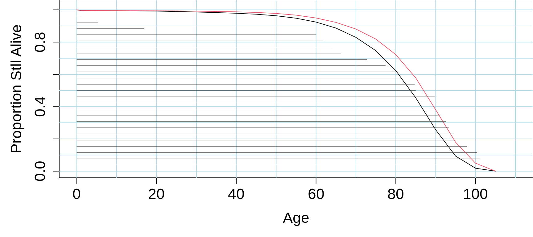
Figure 18.3: Lifetables based on mortality rates of Quebec males (blue) and females(red) in 2018. See above for source of the data. The horizontal 'lifelines' are sorted by length, having been randomly drawn from a simplified survival distribution -- just to illustrate the use of the sort and segments functions in R.
18.2.4 Variable-length (parallel) parking spaces
When setting up parallel parking on city streets, and out of necessity if spaces have individual parking meters, many municipalities use painted rectangles of a fixed dimension. We haven't been able to find universal guidelines for these dimensions -- cities tend to adopt their own, such as the ones here.
Some authorities have pointed to a waste of space when these fixed-size spaces are used. Indeed JH has seen, in Melbourne, Australia, a street where drivers were asked to park in order, starting from the from end of a block, keeping just 1 metre from the car in front, until the entire block filled up.
To see how many additional cars can be accommodated by this scheme, let's compare how this system compares with a fixed-length box of 6.5 meters. Imagine a city block, 130 metres long, that contains \(N\) = 20 fixed-length parking spots. What if it were converted to the 'just fill up from the one end' system with no boundaries? See the example below.
To study this, we have used the most popular makes and models of cars in the UK car-registrations database (déjà vu). For each model, we were able to find its length (in mm) from this database. In instances where the length of a car model changed over time, to reduce the otherwise-lengthy programming and computer-intensive data-extraction, we selected a 'middle' length.
In the resulting data file, each of the 508 rows gives the make and the model, as well as its frequency in the car-registrations database, and its length in millimetres. [The datafile also contains the width, height and mass, which we will use elsewhere to investigate a 'body mass index' for cars]
Read the data into an
R dataframe.Select 25 cars randomly from the just-described frequency distribution, and determine whether, parked a meter apart, they fit into the 130-m long space. Repeat the simulation a sufficient number of times to approach the probablity that this system would provide at least 5 additional spaces.
In a future exercise, we will approach this probability calculation by modelling rather than simulation. Can you imagine what model we will use? Hint: have a look at the distribution (over your simulations) of the total/mean length of 25 randomly selected cars.
This same approach could be used to plan how many people it is safe to have in an elevator that can safely carry a load of say 1000 Km. Does it matter that the shape of the 'weight' distribution has a different shape than the car-lengths distribution? Are there any other factors that come into play here that not present in the car-sampling example? If they are, how will the affect the calculations?
By the way, what shape does the car-lengths distribution have? How would you summarize the distribution?
Suggest ways to measure/who the relation between car-length and popularity.
ds=read.table("http://www.biostat.mcgill.ca/hanley/statbook/DimensionsOfPopularCars.txt",as.is=TRUE)
str(ds)
## 'data.frame': 508 obs. of 6 variables:
## $ Make.Model : chr "ABARTH 500" "ABARTH 595" "ABARTH 695" "ABARTH PUNTO" ...
## $ No.Registered: int 5561 16300 523 703 5059 2503 6444 2268 5327 27605 ...
## $ Length.mm : int 3657 3660 3660 4065 4170 4438 4661 4413 4643 4351 ...
## $ Width.mm : int 1627 1627 1627 1721 1729 1743 1830 1830 1873 1798 ...
## $ Height.mm : int 1485 1485 1485 1478 1442 1430 1422 1372 1436 1465 ...
## $ Weight.Kg : int 1085 1050 1050 1185 1185 1285 1540 1420 1349 1280 ...# plot(ds$Length.mm,log(ds$No.Registered),cex=0.5,pch=19)
N.SIMS=30
LENGTHS = ds$Length.mm/1000
Probs = ds$No.Registered/sum(ds$No.Registered)
E.LENGTH = sum(LENGTHS*Probs)
VAR = sum( (LENGTHS-E.LENGTH)^2 * Probs )
SD = sqrt(VAR)
N = 20
W=6.5
for(n in 20:30){
mu = mean=n*E.LENGTH + n-1
prob.fit = pnorm(N*6.5,mean=mu,sd=sqrt(n)*SD)
#print(round(c(n,E.LENGTH,mu,SD,prob.fit),2))
}
par(mfrow=c(1,1),mar = c(5,5,0,0))
plot(-10,-10,xlim=c(0.5,N+1),ylim=c(0.01,1.01)*N.SIMS,
xlab="Fixed-dimension Parking Spaces",
ylab="Simulation No.",
xaxp=c(1,N,N-1),
cex.axis=1.5,cex.lab=1.5,col="white")
abline(v=1/2 + 0:N,lwd=0.75,col="lightblue")
gaps=(0:(n-1))/W
n = N
for(sim in 1:N.SIMS){
lengths = sample(LENGTHS,size=n,prob=Probs)/W
ends = gaps+cumsum(lengths)
starts = ends - lengths
arrows(starts+1/2, rep(sim,n),
ends+1/2, rep(sim,n),col="blue",
lwd =1.25,
length=0.05,angle=20, code=1
)
starts = 0:(n-1)
ends = starts+lengths
arrows(starts+1/2, rep(sim-0.35,n),
ends+1/2,
rep(sim-0.35,n),col="red",
lwd =1.25,
length=0.05,angle=20, code=1)
}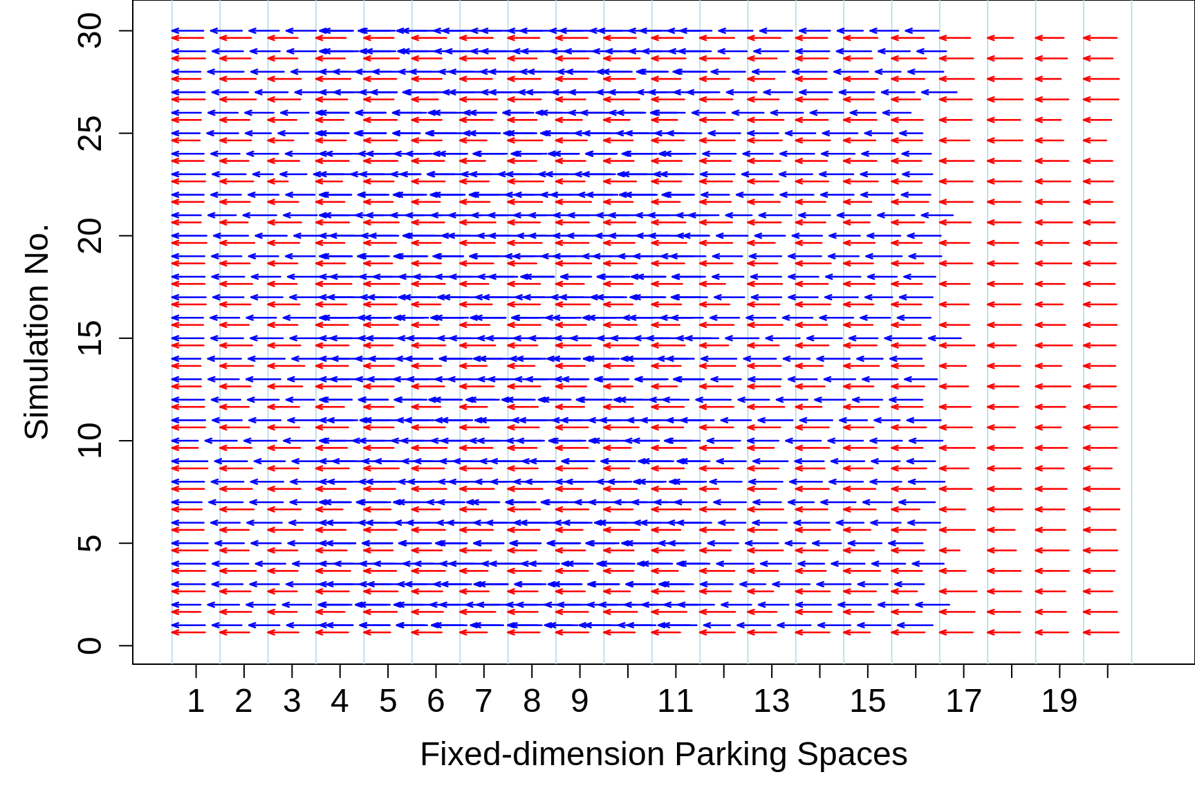
Figure 18.4: 30 simulations of the possible gains from using variable-length (parallel) parking spaces. Shown are 20 fixed-length spaces, each of length 6.5m. In each simulation, 20 cars are selected randomly from the just-described frequency distribution, and their lengths are shown as red lines within the fixed-length parking spaces, and as blues lines, with 1m spacing, in the variable-length scheme.
18.2.5 Galton's data on family heights
The background to these data can be found here
So that he could combine the father's and mother's heights into a single 'mid-parent' height, against which to correlate the offspring height, Francis Galton was keen to establish that height plays a very small part in marriage selection.
Here are the heights of 205 sets of parents, with families numbered 1-135, 136A, 136-204. They are takem directly from his notebook. [See JH's notes on why 7 families are ommitted. Several authors have since extracted the data from JH's webiste, but some (e.g. the authors of the mosaic package) extracted the incomplete version. The Galton dataset in the HistData package has all of the families.]
Categorize each father's height into one of 3 subgroups (shortest 1/4, middle 1/2, tallest 1/4). Do likewise for mothers. Then, as Galton did, obtain the 2-way frequency distribution and visually assess whether you agree with the conclusion "we may therefor regard... " he draws following his Table 9
Calculate the variance Var[F] and Var[M] of the fathers' [F] and mothers' [M] heights respectively. Then create a new variable consisting of the sum of F and M, and calculate Var[F+M]. Comment. Galton called this a "shrewder" test than the "ruder" (coarser) one he used in 1. If the two were unrelated (this is a stronger quality than 'uncorrelated'), what would you expect? If the variance of the sum is greater than the sum of the variances of the parts, what does it suggest.
What if he had subtracted them and calculated the variance of the differences?
When Galton first analyzed these data in 1885-1886, Galton and Pearson hadn't yet invented the correlation coefficient. Calculate this coefficient and see how it compares with your impressions in 1 and 2.
Compare this correlation with the correlation between parental ages in the Penrose dataset.
18.2.6 Height differences of random M-F pairs
Some new-to-statistics (and even some not so new-to) students reason that because the average male is 4-5 inches taller than the average female, the heights of randomly formed M-F pairs would be positively correlated.
In Galton's parental data, in how many of the couples was the man the taller member of the couple?
If you scrambled his data, so as to pair a random father with a random mother, how often would this be the case? you would need to do it several times to get a sense of the proportion.
Explain to these new-to-statistics students why their high correlation based on 4-5 inch average difference is not correct.
Instead of simulating this probability, how otherwsie would you arrive at the probability/propprtion? If you chose to use a 'model', to do so, address the issue of how critical your assumptions are, and whether this approach is robust.
data from NHIS on this topic
caveats.
why did Pearson get correlations that were so much stronger.
https://fivethirtyeight.com/features/how-common-is-it-for-a-man-to-be-shorter-than-his-partner/
18.2.7 Same-sex or opposite-sex?
This 4-panel exercise is modelled on one JH used in the 607 course in 2001, but now using data from all US births in 2018
The data are in this data.frame, and shown in 4 panels numbered A-D. The birthweights within a panel pertain to infants of the same sex, but different panels may pertain to different sexes.
## 'data.frame':    400 obs. of  2 variables:
##  $ Panel      : chr  "A" "A" "A" "A" ...
##  $ Birthweight: int  2809 2186 2607 3231 3484 2836 863 3329 3628 3551 ...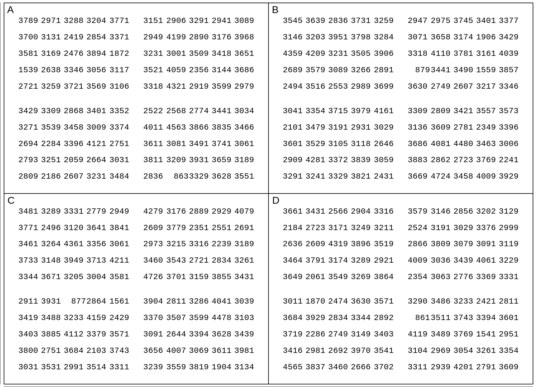
Figure 18.5: Birthweights of US males and females born in 2018. In each panel, each entry is one of the 100 (sex-specific) quantiles Q0.5%, Q1.5%, Q2.5%, Q49.5%, Q50.5%, etc, up to Q99.5%, so you can think of it as representing 1 percent of the births of that sex. In each panel, the Q's are scrambled.
By eye, by comparing all the entries in one panel with all of those in another, you may be able to discern if two panels have different means (or medians). But what can you conclude if you take just a sample from each of 2 panels and perform a formal null hypothesis test using the difference in the sample means or the sample medians, or the ranks?
In 2001, students were asked to perform tests of the following 4 (obviously overlapping, so not completely independent) contrasts:
- \(\mu_A\) vs. \(\mu_B\) \(\quad\) 2. \(\mu_C\) vs. \(\mu_D\) \(\quad\) 3. \(\mu_A\) vs. \(\mu_D\) \(\quad\) 4. \(\mu_B\) vs. \(\mu_C\)
They were asked to use new (fresh, independent) samples of size \(n\) = 4 and \(n\) = 4 for each of the 4 tests.
These sample sizes will (rightly) strike you as being much too small to reliably distinguish two populations whose means are not that far apart. Indeed, most of the students in 2001 were unable to correctly identify the opposite-sex panels
But, when it comes to distinguishing same-sex panels from opposite-sex panels of adult heights, most of the students in 2001 were able to correctly identify the opposite-sex panels, with only a few mistaking the same-sex panels for opposite-sex ones [we are in charge of controlling the latter errors, whereas (with \(n\) fixed) Nature is in charge of the success rate with the former].
Although it isn't realistic, students -- like so many textbooks start with -- were told that the Population Standard Deviation (\(\sigma\)) was known. The main reason for being allowed this 'inside knowledge' (typically reserved for Gods and Oracles) was that it made the computation of the (z-) test statistic easier: students only had compute the two sample means, easily done by hand, and avoided having to compute sample standard deviations. [It also fits with the practice of teaching the simpler z-tests, with their fixed quantiles, first, and then moving to the sample-size-dependent t-based quantiles later]. For now, we will do the same, but later will also go on and carry out real-world tests that don't rely on 'inside' information about standard deviations. [After all, if you know the Population Standard Deviation, then you must already know the Population Mean.]
'ARITHMETIC' of Testing if panels '1' and '2' have same mean
Null Hypothesis: H\(_0: \ \mu_1 = \mu_2\) [same sex, or, technically speaking, same mean]
Alternative Hypothesis H\(_{alt}: \mu_1 \ne \mu_2\) [different means, thus opposite sexes]
Data: sample means \(\bar{y}_1\) and \(\bar{y}_2,\) bases on sample sizes \(n_1\) and \(n_2\)
Test Statistic: \[z = (\bar{y}_1- \bar{y}_2) / SD[\bar{y}_1 - \bar{y}_2],\] where \[SD[\bar{y}_1 - \bar{y}_2] = \sqrt{\sigma^2_1/n_1 + \sigma^2_2/n_2} \ .\]
Probability, P that, under \(H_0\), the test statistic would exceed the absolute value of the observed \(z\) statistic. [the absolute value is used when H\(_{alt}\) is '2-sided'.]
Pre-specified probability, \(\alpha\), below which H\(_0\) is 'rejected'. [by convention, it is often taken to be 0.05; we will use \(\alpha\) = 0.10, so that our simulations are almost sure to yield some 'false positives']
In the case where \(n_1 = n_2 = 4\), and \(\sigma_1\) and \(\sigma_2\) are known, we can work out ahead of time what minimum difference between \(\bar{y}_1\) and \(\bar{y}_2\) would lead us to reject the null (same-sex, or same mean) hypothesis. With \(\alpha\) = 0.10, the 'critical value of \(z\) is \(\pm\) 1.645, i.e, the two sample means would need to be at least 1.645 \(\times SD[\bar{y}_1 - \bar{y}_2]\) apart.
In this simplified and somewhat unrealistic example, where we don't know if we are in the same-sex or opposite sex scenario, we don't know whether we should use \(\sigma_F\) = 574 grams and \(\sigma_M\) = 600 grams, or 574 and 574, or 601 and 601. So we will use a 'compromise' \(\sigma_1\) = \(\sigma_2\) = 587. Substituting these into the \(SD[\bar{y}_1 - \bar{y}_2]\) formula yields an SD of \(\sqrt{587^2/4 + 587^2/4}\) = 415 grams. Thus the critical distance between the two sample means needs to be 1.645 \(\times\) 415 = 683 grams.
For interest, here is what the critical distance would be for other sample sizes: \(n_1 = n_2 = 16:\) 341 grams; \(n_1 = n_2 = 64:\) 171 grams; \(n_1 = n_2 = 256:\) 85 grams. [Notice the root of n law in action.]
Whereas, as an individual 'investigator', you might be luck or unlucky in which of the 4 comparisons you get right, the real issue is the probabilities of getting them right. In 2001 JH had each student in the large 607 class try to distinguish the panels, and he tabulated their results so that we can get a better sense of what these probabilities are. And better still, in 2020, you alone can use the computer to get an even better sense.
We will use the same 2 x 2 table used in 2001, where the 2 rows are the 2 truths, i.e, the comparions was in fact a same-sex or opposite-sex comparison, and the 2 columns are the two possible 'results' of the statistical test, i.e., it was 'negative', with a P-value \(\ge\) 0.1, (the diffrence in the sample means was not 'statistically significant') ; or 'positive' with a P-value \(<\) 0.1, the difference was 'statistically significant', large enough that the null hypothesis of same-sex populations (same-population-means) was 'rejected'.
When you review each test result, you can only classify it by column, by 'negative' or 'positive'. And in real life, that would be as far as you can go, since your are not privy to the 'truth'. But, here, we have the luxury of knowing which comparisons are of each type, so we can cross-classify the results, and also examine the average performance of these tests over many may applications. In this way, we get a feel for the probabilities that they will perfrtom they way we want them to, and can see how the probabilities are modified by the amount of effort (sample size) we are willing to employ, as well as how small/large a signal, and how small/large the noise, we are up against.
So, for now, in your one set of 4 hand-worked examples, you can put the 4 test results into two columns. Below, when we will do a large number of tests, we will reveal which comparisons are of which type, so you can doubly-classify them.
Exercises
- For each of the 4 contrasts listed above, use a 'reproducible' random selection method to choose 4 infants from each of the two specified panels. [Note: since each entry represents almost 200,000 infects, the sampling from the 100 values (quantiles) should be with replacement. This may not matter a lot when you are sampling just 4 infants, but if you were sampling 16 or 64 or 256, it would matter]. For each contrast, compute the difference between the sample means and note whether it was a 'statistically significant' difference (i.e. one of 683 grams or more. These 4 'test tesults' can be the first entries in your 2 x 2 table below, once the identity of each 4 panel (the 'truth') is revealed.
(2-way) distribution of results of statistical tests [columns] in relation to real situations[rows]
| Test Result | Total | ||||
|---|---|---|---|---|---|
| 'Negative' | 'Positive' | ||||
| \(P \ge 0.1\) | \(P \lt 0.1\) | ||||
| SAME-SEX | \(number\) | \(number\) | |||
| TRUTH | |||||
| OPPOSITE | \(number\) | \(number\) | |||
| ......... | ......... | ......... | |||
| TOTAL | \(no._{neg.}\) | \(no._{pos.}\) | TOTAL |
The following R code can simulate the results obtained by many many investigators. For now, the 'many' is just 40, close to the numbers performed by students in 2001. Although this number can only give a rough idea, using sample sizes of size 4 doesn't look that promising! No matter which contrast, only about 10% of the statistical tests are 'positive'. Since we set the \(\alpha\) value, we expect that about 10% of tests are positive when we are testing two same-sex panels, but we would hope that a far greater % would be positive when we are testing opposite-sex panels.
SimulateOppositeSexTests= function(Values,
        n.simulated.investigations = 40,
        n = 4,
        SD.individuals = 583,
        contrasts =
          t(matrix(c("A","B", "C","D","A","D","B","C"),2,4)) ) {

   n.contrasts = dim(contrasts)[1]

   # n.simulated.investigations   per contrast  *** MODIFY ***
   # n =  sample size from each of 2 contrasted panels *** MODIFY ***

   results = matrix(NA,n.simulated.investigations,n.contrasts)

   alpha=0.10 # set by us

   # SD.individuals = xxx,  not usual to KNOW the population SD

   SD.Mean.diff = SD.individuals * sqrt(1/n+1/n) # variance(diff) = Sum of Vars.

   critical.diff = abs( qnorm(alpha/2) * SD.Mean.diff )
   #print( aggregate(Values, by=list(P=ds$Panel), mean) )
   #print( aggregate(Values, by=list(P=ds$Panel), sd) )
   for(i in 1:n.simulated.investigations){
        for (j in 1:n.contrasts){
              pair = contrasts[j,]
              sample.mean = rep(NA,2)
              for(pair.member in 1:2){
                    all.values.this.panel = Values[
                         ds$Panel==pair[pair.member] ]
                    sample.mean[pair.member] =
                         mean( sample(x=all.values.this.panel,
                            size=n, replace = TRUE)    )
              }
              difference = sample.mean[1] - sample.mean[2]
              sig.difference = ( abs(difference) > critical.diff )
              results[i,j] = sig.difference
         } # end of contrasts
    } # end of investigation

    txt = paste("/",toString(n.simulated.investigations))

    DIGITS = ceiling(log(n.simulated.investigations,base=10))
    positives = format( apply(results,2,sum), digits = DIGITS)

    cat(paste("samples of size:",toString(n)))

    noquote( cbind( contrasts[,1],rep(" vs. ",n.contrasts),
                contrasts[,2], rep("  ",n.contrasts), positives,
                rep(txt,n.contrasts)  ) )

} # end functionSimulateOppositeSexTests(ds$Birthweight,
n.simulated.investigations = 50,
n = 4,
SD.individuals = 583,
contrasts =
t(matrix(c("A","B", "C","D","A","D","B","C"),2,4)))## samples of size: 4## positives
## [1,] A vs. B 4 / 50
## [2,] C vs. D 6 / 50
## [3,] A vs. D 7 / 50
## [4,] B vs. C 2 / 50Exercises - continued
Cross-classify the above results into the following 2 x 2 table, knowing which pairs of panels are same-sex and which are opposite-sex to tell you which row of the table a contrast belong to.
Run the
R codeyourself, but with a much larger number of simulated investigations. Cross-classify your results. Even though you know there must be some non-zero difference in the sex-specific means population means, why are the results so dismal? See also the results in 2001.How much better is the performance if you increase the \(n\) to 64? 256?
(2-way) distribution of results of statistical tests [columns] in relation to real situations[rows]
| Test Result | Total | ||||
|---|---|---|---|---|---|
| 'Negative' | 'Positive' | ||||
| \(P \ge 0.1\) | \(P \lt 0.1\) | ||||
| SAME-SEX | \(number\) | \(number\) | |||
| TRUTH | |||||
| OPPOSITE | \(number\) | \(number\) | |||
| ......... | ......... | ......... | |||
| TOTAL | \(no._{neg.}\) | \(no._{pos.}\) | TOTAL |
Exercises - continued
CAN YOU TELL THE GROWN-UPS APART?
The following panels are 100 sex-specific quantiles of weight (kg) of the US Population aged 20-29 years in 2007 to 2008, based on NHANES surveys. JH used interpolation (and a small bit of extrapolation at the lower edges) to create the 100 quantiles, \(Q_{0.005}\), \(Q_{0.015}\), \(\dots\) \(Q_{0.995}\).
Aagin, they are identified as A-D, with the weights within a panel pertain to 20-29 year olds of the same sex, but different panels may pertain to different sexes. The layout is not necessarily the same as it was above for birthweights!
- Cross-classify the above results into the following 2 x 2 table, knowing which pairs of panels are same-sex and which are opposite-sex to tell you which row of the table a contrast belong to.
## 'data.frame':    400 obs. of  2 variables:
##  $ Panel    : chr  "A" "A" "A" "A" ...
##  $ Weight.Kg: num  62.5 47.5 113.5 149.5 108.5 ...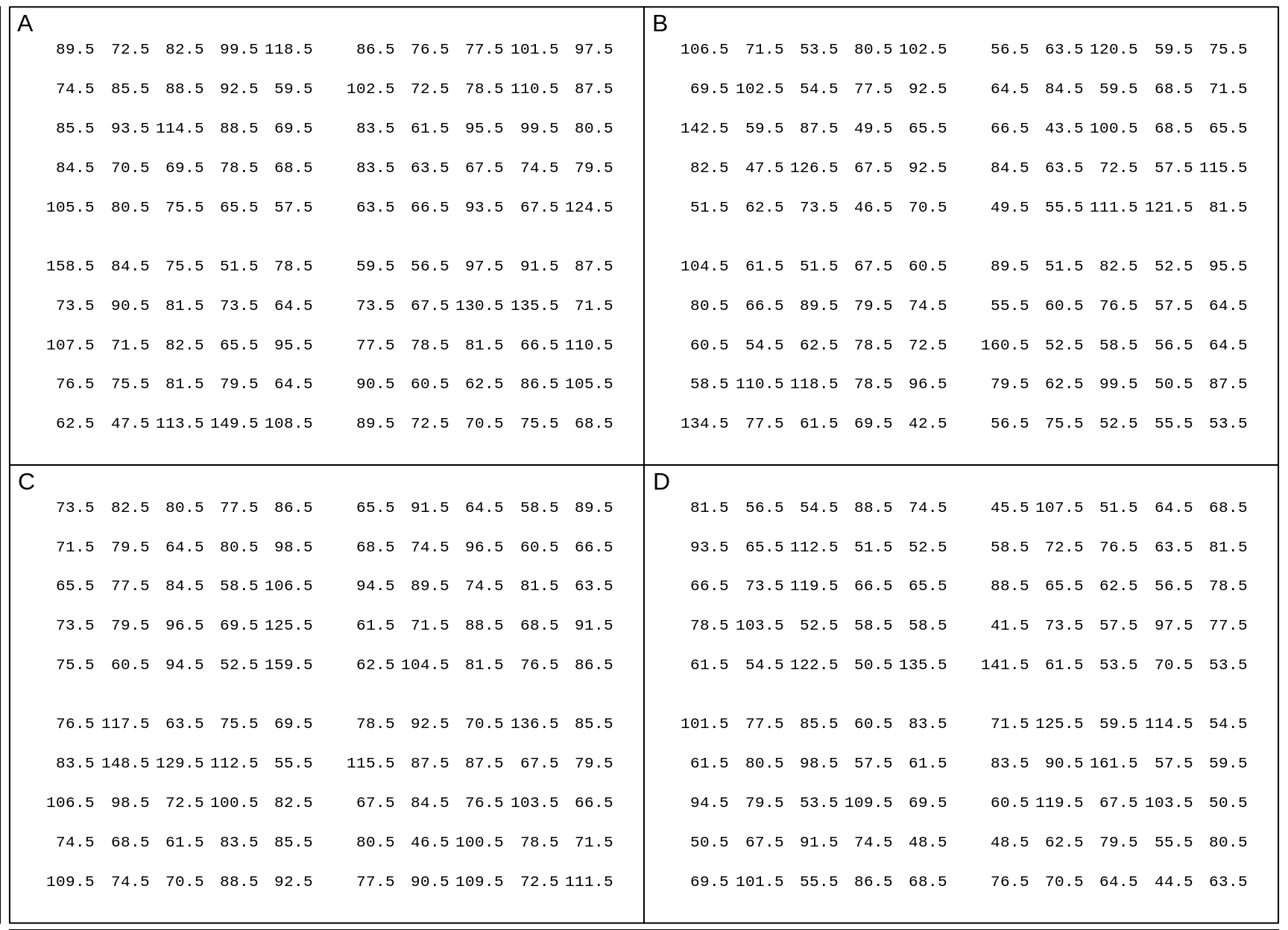
Figure 18.6: Measured weights of US males and females aged 20-29 in 2007-2008. In each panel, each entry is one of the 100 (sex-specific) quantiles Q0.5%, Q1.5%, Q2.5%, Q49.5%, Q50.5%, etc, up to Q99.5%, so you can think of it as representing 1 percent of the population of that sex. In each panel, the Q's are scrambled, and 'jittered'.
By eye, by comparing all the entries in one panel with all of those in another, you can readily tell if two panels have different means (or medians). But what can you conclude if you take just a sample of size 4 from each of 2 panels and perform a formal null hypothesis test using the difference in the sample means or the sample medians, or the ranks?
Exercises - continued
Your are asked to perform tests of the following 4 contrasts:
- \(\mu_A\) vs. \(\mu_C\) \(\quad\) 2. \(\mu_B\) vs. \(\mu_D\) \(\quad\) 3. \(\mu_A\) vs. \(\mu_D\) \(\quad\) 4. \(\mu_B\) vs. \(\mu_C\)
using new (fresh, independent) samples of size \(n\) = 4 and \(n\) = 4 for each of the 4 tests.
- NB: 1 and 2 are not the same as 1 and 2 for birthweight above.
Start by manually performing the 4 tests. Begin by calculating what the critical distance between the two sample means needs to be. Use a 'common' \(\sigma\) = 21.4 Kg for each sex. [Again, it should be obvious why having this 'insider' information is not realistic! It is just to simplify the test to its essentials; later, in practice, we will use 'plug-in' values instead of the 'real' \(\sigma\) and use a larger (\(n\)-based) multiplier to allow for using 'estimated', and thus 'uncertain', \(\sigma\)'s.] How confident are you in the results of these tests? (Remember, you KNOW that males are heavier than females; that is 'prior' information that the test doesn't know: it just uses the data you give it.)
Run the same
R codeyou ran above, with a large number of simulated investigations. In real life, you don't get to see 'what might have been'; you just get to see the one pair of samples you selected. But here the (simulated) 'long-run' perfomance gives you sense of how sensitive your test procedure is [you already know how specific it is, by your choice of \(\alpha\)]. Then, using this key cross-classify your results. How much better did the test do here, than it did with birthweights? Even though the \(n\)'s are still just 4 each, why are they better?
SimulateOppositeSexTests(ds$Weight.Kg,
        n.simulated.investigations = 50,
        n = 4,
        SD.individuals = 21.4,
        contrasts =
          t(matrix(c("A","C", "B","D","A","D","B","C"),2,4)))
## samples of size: 4## positives
## [1,] A vs. C 9 / 50
## [2,] B vs. D 8 / 50
## [3,] A vs. D 13 / 50
## [4,] B vs. C 5 / 50CAN YOU TELL THE 20-SOMETHINGS APART BY THEIR HEIGHTS?
ds = read.table(
  "http://www.biostat.mcgill.ca/hanley/statbook/USheights100Qs20072008.txt",
  as.is=TRUE)
str(ds)
## 'data.frame': 400 obs. of 2 variables:
## $ Panel : chr "A" "A" "A" "A" ...
## $ Height.cm: int 175 173 168 181 186 189 179 171 161 169 ...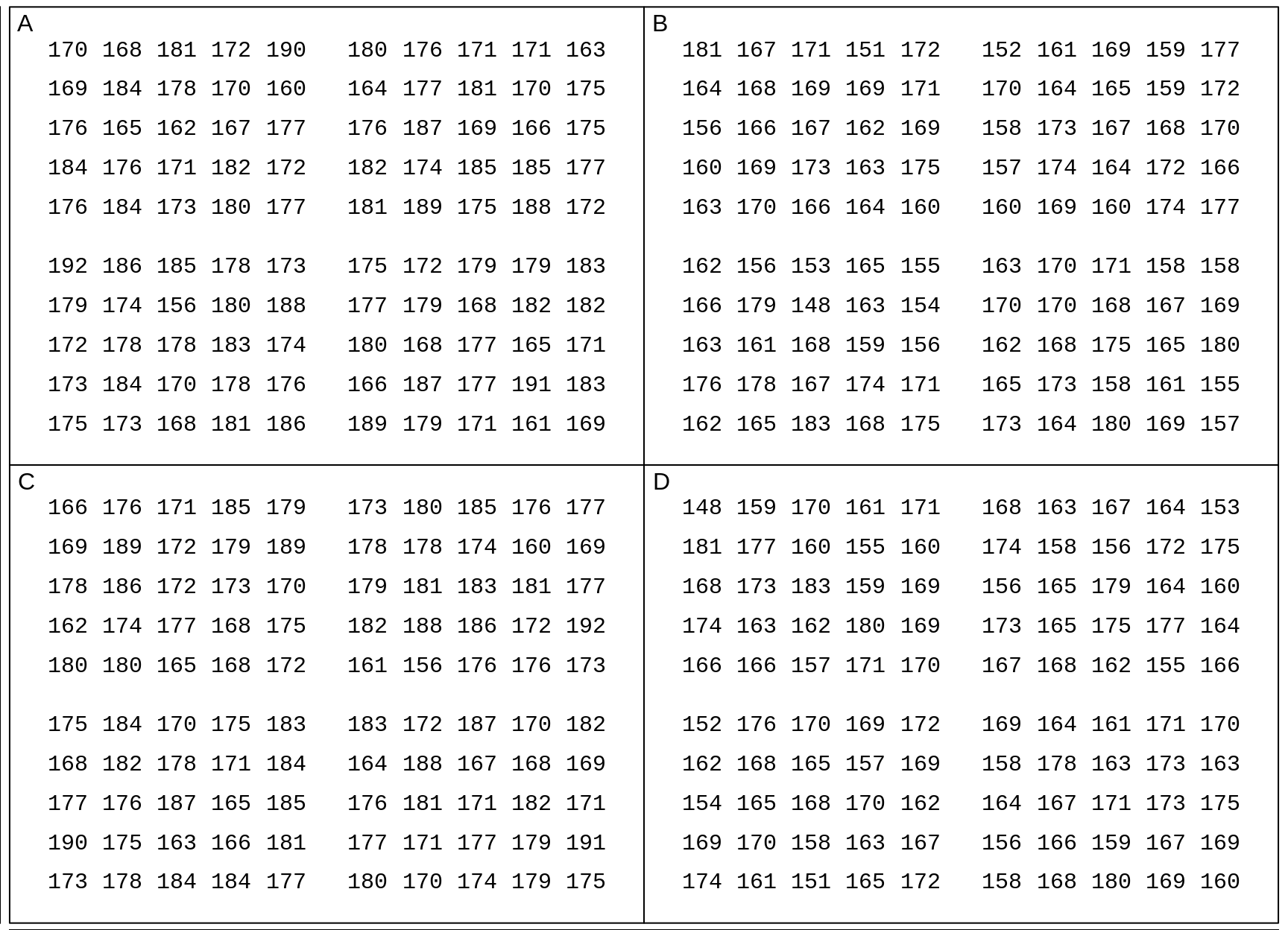
Figure 18.7: Measured heights (in cm) of US males and females aged 20-29 in 2007-2008. In each panel, each entry is one of the 100 (sex-specific) quantiles Q0.5%, Q1.5%, Q2.5%, Q49.5%, Q50.5%, etc, up to Q99.5%, so you can think of it as representing 1 percent of the population of that sex. In each panel, the Q's are scrambled.
Here are the test results
SimulateOppositeSexTests(ds$Height.cm,
        n.simulated.investigations = 50,
        n = 4,
        SD.individuals = 7.3,
        contrasts =
          t(matrix(c("A","C", "B","D","A","D","B","C"),2,4)))
## samples of size: 4## positives
## [1,] A vs. C 9 / 50
## [2,] B vs. D 5 / 50
## [3,] A vs. D 32 / 50
## [4,] B vs. C 32 / 50Exercises - continued
Using the (common) SD of 7.3 cm, carry out 4 manually-calculated tests of the same 4 contrasts as for adult weights.
(although the computer-simulated ones are giving you a sense that height is a more sensitive distinguisher/separator of the sexes than adult weight is, carry out a larger set of simulated tests to be sure.
Statistically speaking, why is height a more sensitive distinguisher/separator of the sexes? Hint: how far apart are the mean heights (a) in cms (b) as a percentage of the SD of the individuals of a given sex? What are the corresponding perecenatges in the case of birthweights? adult weights? What we are fetting at here is the signal-to-noise ratio or Effect Size \[ \frac{Signal}{Noise} = \frac{\mu_1 - \mu_2}{\sigma}.\]
In 2001, when it came to distinguishing same-sex panels from opposite-sex panels of adult heights, a clear majority (63/76) of the students were able to correctly identify the opposite-sex panels, with only a few (8/75) mistaking the same-sex panels for opposite-sex ones. To try to answer why we do not do as well with our data, compute the sex-specific means and SD's of the 100 quantiles, and compare the effect sizes with those in 2001. You might also make boxplots to see if the shapes of the data differ [JH doesn't remember how he made the 100 values in 2001, but for sure the ones above are closer to the real shapes.] To save you manually extracting them, the data from 2001 can be found here.
Statistically speaking, why are the 'false positive rates' about the same with the new data and the 2001 data. Hint: Who determines them?
Biologically speaking, why is adult height a more sensitive distinguisher/separator of the sexes than adult weight? Hint: think about the relative roles of Nature and Nurture -- and while you are on this topic, look up the origins of the Nature versus Nurture phrase.
18.2.8 Box minus bowl
18.2.9 car parking fixed and variable
18.2.10 Correcting length-biased sampling
=====================
18.3 Other Exercises (under construction)
Exercises
Variation with and without constraints Pearson vs Fisher
Ice Breakup Dates
Here are some details on the Nenana Ice Classic More here
18.3.1 The 2018 Book of Guesses
We are keen to establish the distribution of guesses, with the guessed times measured from midnight on December 31, 2017. Thus a guess of April 06, at 5:15 p.m. would be measured as 31 + 28 + 31 + 5 + 12/24 + (5+ 15/60)/24 = 95.71875 days into the year 2018.
It would be tedious to apply optical character recognition (OCR) to each of the 1210 pages in order to be able to computerize all 240,000 guesses. Instead, you are asked to reconstruct the distribution of the guesses in two more economical ways:
By determining, for (the beginning of) each day, from April 01 to June 01 inclusive, the proportion, p, of guesses that predede that date. [ In
R, if p = 39.6% of the guesses were below 110 days, we would write this as pGuessDistribution(110) = 0.396. Thus, if we were dealing with the location of a value in a Gaussian ('normal') distribution, we would writepnorm(q=110, mean = , sd = )] Once you have determined them, plot these 62 p's (on the vertical axis) against the numbers of elapsed days (90-152) on the horizontal axis.By determining the 1st, 2nd, ... , 98th, 99th percentiles. These are specific examples of 'quantiles', or q's. The q-th quantile is the value (here the elapsed number of days since the beginning of 2018) such that a proportion q of all values are below this value, and 1-q are above it. [ In
R, if 40% of the guesses were below 110.2 days, we would write this as qGuessDistribution(p=0.4) = 110.2 days. Thus, if we were dealing with the 40th percentile of a Gaussian distribution with mean 130 and standard deviation 15, we would writeqnorm(p=0.4, mean = 130, sd = 15). ] Once you have determined them, plot the 99 p's (on the vertical axis) against the 99 (elapsed) times on the horizontal axis.Compare the Q\(_{25}\), Q\(_{50}\), and Q\(_{75}\) obtained directly with the ones obtained by interpolation of the curve showing the results of the other method.
Compare the directly-obtained proportions of guesses that are before April 15, April 30, and May 15 with the ones obtained by interpolation of the curve showing the results of the other method.
By successive subtractions, calculate the numbers of guesses in each 1-day bin, and make a histogram of them. From them, calculate the mean, the mode, and the standard deviation.
To measure the spread of guesses, Galton, in his vox populi (wisdom of crowds) article, began with the interquartile range (IQR), i.e. the distance between Q75 and Q25, the 3rd and 1st quartiles. In any distribution, 1/2 the values are within what was called the 'probable error (PE) of the mean; i.e., it is equally probable that a randomly selected value would be inside or outside this middle-50 interval. Today, we use standard deviation (SD) instead of probable error. In a Gaussian distribution, some 68% of values are within 1 SD of the mean, whereas 50% of values are within 1 PE of the mean. We can use R to figure out how big a PE is in a Gaussian distribution compared with a SD. By setting the SD to 1, and the eman to 0, we have
Q75 = qnorm(p = 0.75, mean=0, sd=1)
round(Q75,2)
## [1] 0.67i.e, a PE is roughtly 2/3rds of a SD.
Galton -- convert to SD.
Geometric mean Amsterdam study
How far off was the median guess in 2018 from the actual time? Answer in days, and (with reservations stated) as a percentage?
Why did the experts at the country fair do so much better?
Where were the punters in 2019 wrt the actual ?
https://www.all-about-psychology.com/the-wisdom-of-crowds.html
http://galton.org/essays/1900-1911/galton-1907-vox-populi.pdf
[Nenana Ice Classic]
Tanana River
18.3.2 Trends over the last 100 years
fill in the data since 200x.
cbind with ...
time trends
morning vs afternoon ?
2019 extreme... how many SD's from the line?
- Where were the punters in 2019 wrt the actual ?
Sources:
1917-2003 data in textfile on course website;
http://www.nenanaakiceclassic.com/ for data past 2003
ascii (txt) and excel files with data to 2003
Working in teams of two ...
*Create a dataframe containing the breakup data for the years 1917-2007. Possible ways to do so include: directly from the ascii (txt) file; from the Excel file
*From the decimal portion of the Julian time, use R to create a frequency table of the hour of the day at which the breakup occurred.
*From the month and day, use R to calculate your own version of the Julian day (and the decimal portion if you want to go further and use the hour and minute)
*Is there visual evidence that over the last 91 years, the breakup is occurring at an earlier date?
*Extract the date and ice thickness measurements for the years 1989-2007 from the website and use (your software of choice) R to create a single dataset with the 3 variable, year, day and thickness. From this, fit a separate trendline for each year, and calculate the variability of these within-year slopes.
- Galton’s data on family heights
These data were gathered to examine the relation between heights of parents and heights of their (adult) children. They have been recently 'uncovered' from the Galton archives. As a first issue, for this exercise, you are also asked to see whether the parent data suggest that stature plays "a sensible part in marriage selection”.
For the purposes of this exercise, the parent data [see http://www.epi.mcgill.ca/hanley/galton ] are in a file called parents.txt , with families numbered 1-135, 136A, 136-204 ( {the heights of the adult offspring will be used in a future exercise)
Do the following tasks using R
Categorize each father's height into one of 3 bins (shortest 1/4, middle 1/2, tallest 1/4). Do likewise for mothers. Then, as Galton did [ Table III ], obtain the 2-way frequency distribution and assess whether "we may regard the married folk as picked out of the general population at haphazard".
Calculate the variance Var[F] and Var[M] of the fathers' [F] and mothers' [M] heights respectively. Then create a new variable consisting of the sum of F and M, and calculate Var[F+M]. Comment. Galton called this a "shrewder" test than the "ruder" one he used in 1.
When Galton first anayzed these data in 1885-1886, Galton and Pearson hadn't yet invented the correlation coefficient. Calculate this coefficient and see how it compares with your impressions in 1 and 2.
- Temperature perceptions
Create 5 datasets from the questionnaire data on temperature perceptions etc.
by importing directly from the Excel file applied to .csv version of Excel file);
by first removing the first row (of variable names) and exporting the Excel file into a 'comma-separated-values" (.csv) text file, then ...
reading the data in this .csv file via the INFILE and INPUT statements in a SAS DATA step,
[SAS] INFILE 'path' DELIMITER =","; INPUT ID MALE $ MD $ EXAM TEMPOUTC TEMPINC TEMPOUTF TEMPINF TEMPFEEL TIME PLACE $ ;
- by reading the data in the text file temps_1.txt into
the SAS dataset via the INFILE and INPUT statements. Notice that the 'missing' values use the SAS representation (.) for missing values.
or the Stata dataset using the 'infile' command
- by reading the data in the text file temps_2.txt via [in SAS] the INFILE and INPUT statements in a DATA step or [in Stata] the 'infix' command.
Here you will need to be careful, since 'free-format' will not work correctly (it is worth trying free format with this file, just to see what goes wrong!). When using the INFILE method, you can control some of the damage by using the 'MISSOVER' option in the INFILE statement: this keeps the INPUT statement from continuing on into the next data line in order to find the (in our example) 11 values implied by the variable list. JH uses this 'defensive' option in ALL of his INFILE statements.
- by cutting and pasting the contents of the text file temps_2.txt directly into the SAS or Stata program - in SASthe lines of data go immediately after the DATALINES statement, and there needs to be a line containing a semicolon to indicate the end of the data stream. In Stata, the lines of data go immediately after the infile or infix statement, and there needs to be a line containing the word 'end' to indicate the end of the data stream
This Cut and Paste Method is NOT RECOMMENDED when the number of observations is large, as it is too all too easy to inadvertently alter the data, and the SAS/Stata porogram becomes quite long and unwieldy. It is Good Data Management Practice to separate the program statements from the data.
[Run [in SAS] PROC MEANS [in Stata] the 'describe' command, on the numerical variables, and [in SAS] PROC FREQ or [in Stata] the 'tabulate' command, on the non-numerical variables, to check that the 5 datasets you created contain the same information. Also, get in the habit of viewing or printing several observations and checking the entries against the 'source'.
When using (i), have SAS show you the SAS statements generated by the wizard. Store these, and the DATA steps for (ii) to (v) in a single SAS program file (with suffix .sas).
Annotate liberally using comments:
in SAS, either begin with * ; or enclose with /* ... */
in Stata ..begin the line with * or place the comment between /* and */ delimiters or begin the comment with // or begin the comment with ///
Q2
Use one of these 5 datasets, and the appropriate [in SAS, PROCs (see Exploring Data under UCLA SAS Class Notes 2.0)], or [in Stata, the list comamnd, and the analyses from the Statistics menu] tolist the names and characteristics of the variables
list the first 5 observations in the dataset
list the id # and the responses just to q3, w5 and q6, for all respondents, with respondents in the order: female MDs, male MDs, female non-MDs, male non-MDs. Indicate the [sub-]statement that is required to reverse this order.
create a 2-way frequency table, showing the frequencies of respondents in each of the 2 (MD nonMD) x 2 (male female) = 4 'cells' (one defintion of an epidemiologist is 'an MD broken down by age and sex'). Turn off all the extra printed output, so that the table just has the cell frequencies and the row and column totals.
compare the mean and median attitude to exams in MDs vs. non-MDs (hint: in SAS, the CLASS statement may help). Get SAS/Stata to limit the output to just the 'n', the min, the max, the mean and the median for each subgroup. And try to also get it to limit the number of decimal places of output (in SAS the MAXDEC option is implememnted in some procedures, but as far as JH can determine not in all)
compare the mean temperature perceptions (q6) of male and female respondents
[in SAS] create a low-res ('typewriter' resolution) scatterplot of the responses to q5 (vertical axis) vs. q4 (horizonatal axis), using a plotting symbol that shows whether the responsdent is a male or a female. If we have not covered how to show this '3rd dimension', look at the ONLINE Documentation file {the guide for most of the procedures covered in this set of exercises is in the Base SAS Procedures Guide; other procedures are in sthe more advanced 'STAT' module}. You can specify the variable whose values are to mark each point on the plot. See PLOT statement in PROC PLOT, and the example with variables height weight and gender. [in Stata] use the (automatically hi-res) graphics capabilities available from the 'Graphics' menu
[if SAS] Put all of the programs for Q1, and all of these program steps and output for Q2 in a single .txt file (JH will use a mono-spaced font such as Courier to view it -- that way the alignment should be OK), with PROC statements interleaved with output, and a helpful 2-line title (produced by SAS, but to your specifications) over top of each output. Get SAS to set up the output so that there are no more that 65 horizontal characters per line (that way, lines won't wrap-around when JH views the material).
[if Stata] paste the results and graphics into Word.
NOTE: To be fair to SAS, it CAN produce decent (and even some publication-quality) graphics. See http://www.ats.ucla.edu/stat/sas/topics/graphics.htm
Then submit the text file electronically (i.e., by email) to JH by 9 am on Monday October 2.
- Natural history of prostate cancer
Q1
The following data items are from an investigation into the natural history of (untreated) prostate cancer [ report (.pdf) by Albertsen Hanley Gleason and Barry in JAMA in September 1998 ].
id, dates of birth and diagnosis, Gleason score, date of last contact, status (1=dead, 0=alive), and -- if dead -- cause of death (see 2b below). data file (.txt) for a random 1/2 of the 767 patients
Compute the distribution of age at diagnosis (5-year intervals) and year of diagnosis (5 year intervals). Also compute the mean and median ages at diagnosis.
For each of the 20 cells in Table 2 (5 Gleason score categories x 4 age-at-dx categories), compute the
number of man-years (M-Y) of observation
number of deaths from prostate cancer(1), other causes(2), unknown causes(3)
prostate cancer(1) death rate [ deaths per 100 M-Y ]
proportion who survived at least 15 years.
For a and b you can use the 'sum' option in PROC means; ie PROC MEANS data = ... SUM; VAR vars you want to sum; BY the 2 variables that form the cross-classification. Also think of a count as a sum of 0s and 1s. For c (to avoid having to compute 20 rates by hand), you can 'pipe' i.e. re-direct the sums to a new sas datafile, where you can then divide one by other to get (20) rates. Use OUTPUT OUT = .... SUM= ...names for two sums;
On a single graph, plot the 5 Kaplan-Meier survival curves, one for each of the 5 Gleason score categories (PROC LIFETEST .. Online help is under the SAS STAT module, or see http://www.ats.ucla.edu/stat/sas/seminars/sas_survival/default.htm. For Stata, see http://www.ats.ucla.edu/stat/stata/seminars/stata_survival/default.htm.
[OPTIONAL] In order to compare the death rates with those of U.S. men of the same age, for each combination of calendar year period (1970-1974, 1975-1979, ..., 1994-1999) and 5 year age-interval (55-59, 60-64, ... obtain
the number of man-years of follow-up and
the number of deaths.
Do so by creating, from the record for each man, as many separate observations as the number of 5yr x 5yr "squares" that the man traverses diagonally through the Lexis diagram [ use the OUTPUT statement within the DATA step]. Then use PROC MEANS to aggregate the M-Y and deaths in each square. If you get stuck, here is some SAS code that does this, or see the algorithm given in Breslow and Day, Volume II, page ___
Put all of the program steps and output into a single .txt file. JH will use a mono-spaced font such as Courier to view it -- that way the alignment should be ok. Interleave DATA and PROC statements with output and conclusions, and use helpful titles (produced by SAS, but to your specifications) over top of each output. Get SAS to set up the output so that there are no more that 65 horizontal characters per line -- that way, lines won't wrap-around even when the font used to view your file is increased. Show relevant excerpts rather than entire listings of datafiles. Annotate liberally. Submit the text file electronically (i.e., by email) to JH by 9 am on Monday Nov 7.
- Serial PSA values
Q1
These two files contain PSA values [pre-] and [post-] treatment of prostate cancer *.
- Create a 'wide' PSA file of 25 log-base-2 PSA values per man (some will be missing, if PSA not measured 25 times). Print some excerpts.
(b)From the dataset created in (a), create a long file, with just the observations containing the non-missing log-base-2 PSA values [OUTPUT statement in DATA step]. Print and plot some excerpts.
- From the dataset created in (b), create a wide file [ RETAIN, first. and last. helpful here; or use PROC TRANSPOSE ]. Print some excerpts.
- The order of the variables is given in this sas program . Some of the code in the program may also be of help.
Put all of the program steps and output into a single .txt file. JH will use a mono-spaced font such as Courier to view it -- that way the alignment should be ok. Interleave DATA and PROC statements with output and conclusions, and use helpful titles (produced by SAS, but to your specifications) over top of each output. Get SAS to set up the output so that there are no more that 65 horizontal characters per line -- that way, lines won't wrap-around even when the font used to view your file is increased. Show relevant excerpts rather than entire listings of datafiles. Annotate liberally. Submit the text file electronically (i.e., by email) to JH by 9 am on Monday Nov 14.
- Graphics
1a
Re-produce (or if you think you can, improve on) three of the graphs shown in "Examples of graphs from Medical Journals." These examples are in a pdf file on the main page. Use Excel for at least one of them, and R/Stata/SAS for at least one other. Do not go to extraordinary lengths to make them exactly like those shown -- the authors, or the journals themselves, may have used more specialized graphics software. You may wish to annotate them by making (and sharing with us) notes on those steps/options that were not immediately obvious and that took you some effort to figure out. Insert all three into a single electronic document.
1b
Browse some medical and epidemiologic journals and some magazines and newspapers published in the last 12 months, Identify the statistical graph you think is the worst, and the one you think is the best. Tell us how many graphs you looked at, and why you chose the two you did. If you find a helpful online guide or textbook on how to make good statistical graphs, please share the reference with us. [The bios601 site http://www.epi.mcgill.ca/hanley/bios601/DescriptiveStatistics/ has a link to the Textbook by Cleveland and the book "R Graphics" by Paul Murrell.
If possible, electronically paste the graphs into the same electronic file you are using for 1a.
2
[OPTIONAL] The main page has a link to a lifetable workbook containing three sheets. Note that the 'lifetable' sheet in this workbook is used to calculate an abridged current life table based on the 1960 U.S. data. Use this sheet as a guideline, and create a current life-table ('complete', i.e., with 1-year age-intervals) for Canadian males, using the male population sizes, and numbers of deaths, by age, Canada 2001. [The calculations in columns O to W of the lifetable sheet are not relevant for this exercise]. Details on the elements of, and the construction of current lifetables can be found in the chapters (on website) from the textbooks by Bradford Hill and Selvin, and in the technical notes provided by the US National Center for Health Statistics in connection with US Lifetable 2000. See also the FAQ for 613 from 2005. The fact that the template is for an abridged life table, with mostly 5-year intervals, whereas the task is to construct a full lifetable with 1 year intervals, caused some people problems last year.. they realized something was wrong when the life expectancy values were way off!
Since this is an exercise, and not a calculation for an insurance company that wants to have 4 sig. decimal places, don't overly fuss about what values of 'a' you use for the early years.. they don't influence the calculations THAT much: If you try different sets of values (such as 0.1 in first year and 0.5 thereafter) you will not find a big impact. But don't take my word for it .. the beauty of a spreadsheet is that you can quickly see the consequences of different assumptions or 'what ifs'.
[In practice, in order not to be unduly influenced by mortality rates in a single calendar year (e.g. one that had a very bad influenza season), current lifetables are usually based on several years of mortality data. Otherwise, or if they are based on a small population, the quantities derived from them will exhibit considerable random fluctuations from year to year ]
Once you have completed the table, use the charting facilities in Excel to plot the survival curve for the hypothetical (fictitious) male 'cohort' represented by the current lifetable.
On a separate graph, use two histograms to show the distributions of the ages at death (i) for this hypothetical male 'cohort' and (ii) those males who died in 2001. To make it easy to compare them, superimpose the histograms or put them 'side by side' or 'back to back' within the same graph. Explain why the two differ in shape and location. Calculate/derive (and include them somewhere on the spreadsheet) the median and mean age at death in the hypothetical cohort and the corresponding statistics for the actual deaths in 2001.
- Possible Body Mass Indices
This exercise investigates different definitions of Body Mass Index (BMI).
BACKGROUND: With weight measured in Kilograms, and height in metres, BMI is usually defined as weight divided by the SQUARE of height, i.e., BMI = Wt / (Height*Height), or BMI = Wt/(height2) using, as SAS and several other programming languages do, the symbol for 'raised to the power of'. [ NB: Excel uses ^ to denote this ]
What's special about the power of 2? Why not a power of 1 i.e., Weight/height?
Why not 3, i.e., Weight/*(height3) ? Why not 2.5 i.e. Weight/(height2.5)?
One of the statistical aims of a transformation of weight and height to BMI is that BMI be statistically less correlated with height, thereby separating height and height into two more useful components height and BMI. For example in predicting lung function (e.g. FEV1), it makes more sense to use height and BMI than height and weight, since weight has 2 components in it -- it is partly height and partly BMI. Presumably, one would choose the power which minimizes the correlation.
The task in this project is to investigate the influence of the power of height used in the ratio, and to see if the pattern of correlations with power is stable over different settings (datasets).
DATA: To do this, use 2 of the 6 datasets on the 678 webpage: [usernane is c678 and p w is H**J44 ]
- Children aged 11-16 Alberta 1985 (under 'Datasets')
- 18 year olds in Berkeley longitudinal study, born 1928/29 (under 'Datasets')
- Dataset on bodyfat -- 252 men (see documentation) (under 'Datasets')
- Pulse Rates before and after Exercise -- Australian undergraduates in 1990's (under 'Projects')
- Miss America dataset 1921-2000 (under 'Resources')
- Playboy dataset 1929-2000 (under 'Resources')
METHODS: First create each of the two SAS datasets, and if height and weight are not already in metres and Kg, convert them to these units. Drop any irrelevant variables. Inside each dataset, create a variable giving the source of the data (we will merge the two -- and eventually all six-- datasets, so we need to be able to tell which one each observation came from).
Combine the two datasets, i.e. 'stack' them one above the other in a single dataset. Print out some excerpts.
For each subject in the combined dataset, create 5 versions of <
Calculate the correlation between the 'BMI' obtained with each of these powers, and height. Do this separately for the observations from the two different sources (the BY statement should help here).
Report your CONCLUSIONS.
- Galton
The objective of this exercise is to examine the relation between heights of parents and heights of their (adult) children, using recently 'uncovered' data from the Galton archives, You are asked to assess if Galton's way of dealing with the fact that heights of males and females are quite different produces sharper correlations than we would obtain using 'modern' methods of dealing with this fact. As side issues, you are also asked to see whether the data suggest that stature plays "a sensible part in marriage selection" and to comment on the correlations of the heights in the 4 {father,son}, {father,daughter}, {mother,son} and {mother,daughter} pairings.
BACKGROUND: Galton 'transmuted' female heights into their 'male-equivalents' by multiplying them by 1.08, and then using a single combined 'uni-sex' dataset of 900-something offspring and their parents. While some modern-day anayysts would simply calculate separate correlations for the male and female offspring (and then average the two correlations, as in a meta-analysis), most would use the combined dataset but 'partial out' the male-females differences using a multivariable analysis procedure. The various multivariable procedures in effect create a unisex dataset by adding a fixed number of inches to each female's height (or, equivalently, in the words of one of our female PhD students, by 'cutting the men down to size'). JH was impressed by the more elegant 'proportional scaling' in the 'multiplicative model' used by Galton, compared with the 'just use the additive models most readiliy available in the software' attitude that is common today. In 2001, he located the raw (untransmuted) data that allows us to compare the two approaches.
DATA: For the purposes of this exercise, the data [see http://www.epi.mcgill.ca/hanley/galton ] are in two separate files:
- the heights# of 205 sets of parents ( parents.txt ) with families numbered 1-135, 136A, 136-204
the heights# of their 900-something* children ( offspring.txt ) with families numbered as above
The data on eight families are deliberately omitted, to entice the scholar in you to get into the habit of looking at (and even double checking) the original data. Since here we are more interested in the computing part in this course, and because time is short, ignore this invitation to inspect the data -- we already had a look at them in class. In practice, we often add in 'missing data' later, as there are always some problem cases, or lab tests that have to be repeated, or values that need to be checked, or subjects who didn't get measured at the same time as others etc.. JH's habit is to make the additions in the 'source' file (.txt or .xls or whatever) and re-run the entire SAS DATA step(s) to create the updated SAS dataset (temporary or permanent). If the existing SAS datset is already large, and took a lot of time to create, you might consider creating a small dataset with the new observations, and then stacking (using SE) the new one under the existing one -- in a new file. SAS has fancier ways too, and others may do things differently!
If your connection is too slow to view the photo of the first page of the Notebook, the title reads
FAMILY HEIGHTS (add 60 inches to every entry in the Table)
METHODS/RESULTS/COMMENTS:
Categorize each father's height into one of 3 subgroups (shortest 1/4, middle 1/2, tallest 1/4). Do likewise for mothers. Then, as Galton did [ Table III ], obtain the 2-way frequency distribution and assess whether "we may regard the married fold as picked out of the general population at haphazard".
Calculate the variance Var[F] and Var[M] of the fathers' [F] and mothers' [M] heights respectively. Then create a new variable consisting of the sum of F and M, and calculate Var[F+M]. Comment. Galton called this a "shrewder" test than the "ruder" one he used in 1. ( statistic-keyword VAR in PROC MEANS)
When Galton first anayzed these data in 1885-1886, Galton and Pearson hadn't yet invented the CORRelation coefficient. Calculate this coefficient and see how it compares with your impressions in 1 and 2.
Create two versions of the transmuted mother's heights, one using Galton's and one using the modern-day (lazy-person's, blackbox?) additive scaling [for the latter, use the observed difference in the average heights of fathers and mothers, which you can get by e.g., running PROC MEANS on the offspring dataset, either BY gender, or using gender as a CLASS variable]. In which version of the transmuted mothers' heights is their SD more simlar to the SD of the fathers? ( statistic-keyword STD in PROC MEANS)
Create the two corresponding versions of what Galton called the 'mid-parent' (ie the average of the height of the father and the height of the transmuted mother). Take mid-point to mean the half-way point (so in this case the average of the two)
Create the corresponding two versions (additive and multiplicative scaling) of the offspring heights (note than sons' heights remain 'as is'). Address again, but now for daughters vs sons, the question raised at the end of 4.
Merge the parental and offspring datasets created in steps 4 and 6, taking care to have the correct parents matched with each offspring (this is called a 1:many merge).
Using the versions based on 1.08, round the offspring and mid-parent heighs to the nearest inch (or use the FLOOR function to just keep the integer part of the mid-parent height --you need not be as fussy as Galton was about the groupings of the mid-parent heights), and obtain a 2-way frequency distribution similar to that obtained by Galton [ Table I ]. Note that, opposite to we might do today, Galton put the parents on the vertical, and the offspring on the horizontal axis. ( The MOD INT FLOOR CEIL and ROUND functions can help you map observations into 'bins' ; we will later see a way to do so using loops)
Galton called the offspring in the same row of his table a 'filial array'. Find the median height for each filial array, and plot it, as Galton did, against the midpoint of the interval containing their midparent -- you should have one datapoint for each array. Put the mid-parent values on the vertical, and the offspring on the horizontal axis. By eye, estimate the slope of the line of best fit to the datapoints. Mark your fitted line by 'manually' inserting two markers at the opposite corners of the plot. Does the slope of your fitted line agree with Galton's summary of the degree of "regression to mediocrity"? [ Plate IX ] Note that Galton used datapoints for just 9 filial arrays, choosing to omit those in the bottom and top rows (those with the very shortest and the very tallest parents) because the data in these arrays were sparse. ( By using the binned parental height in the CLASS statement in PROC MEANS or PROC UNIVARIATE, directing the output to a new SAS dataset, and applying PROC PLOT to this new dataset, you can avoid having to do the plotting manually See more on this in the FAQ)
Plot the individual unisex offspring heights (daughters additively transmuted) versus the mid-parent height (mothers transmuted). OVERLAY on it, with a different plotting symbol, the corresponding plot involving the multiplicatively transmuted offspring values (on the parent-axis, stay with Galton's definition of a midparent). (see FAQ) Compare the two, and have a look at Galton's fitted ellipse, corresponding to a bivariate normal distribution [ Plate X ]) {here, again, we would be more likely to plot the parents' heights on the horizontal, and the offspring heights on the vertical axis}.
For each of the following 'offspring vs. mid-parent' correlations, use the 'mid-parent' obtained using Galton's multiplicative method. Calculate (a) the 2 correlations for the 2 unisex versions of the offspring data (b) the sex-specific correlations (i.e., daughters and sons separately) and (c) the single parent-offspring correlation, based on all offspring combined, and their untransmuted heights, ignoring the sex of the offspring. Comment on the correlations obtained, and on the instances where there are big disparities between them. [ a PLOT, with separate plotting symbols for sons and daughters, might help in the case of (c) ]
Calculate the 4 correlations (i) father,son (ii) father,daughter, (iii) mother,son and (iv) mother,daughter. Comment on the pattern, and on why you think it turned out this way.
Put all of the program steps and output into a single .txt file. JH will use a mono-spaced font such as Courier to view it -- that way the alignment should be ok. Interleave DATA and PROC statements with output and conclusions, and use helpful titles (produced by SAS, but to your specifications) over top of each output. Get SAS to set up the output so that there are no more that 65 horizontal characters per line -- that way, lines won't wrap-around even when the font used to view your file is increased. Show relevant excerpts rather than entire listings of datafiles. Annotate liberally. Submit the text file electronically (i.e., by email) to JH by 9 am on Monday October 30.
Lottery payoffs
sampling of children in school
Detecting a fake Bernoulli sequence
Cell occupancy