Chapter 17 Computing: Session No. 3
17.1 Objectives
The 'computing' objective is to learn how to use R to evaluate probabilities by (Monte Carlo) simulation. Taks, and the R Functions/structures used include
taking a sample of a specified size from the elements of a vector, either with or without replacement:
sample,creating a matrix from the given set of values:
matrix,forming a vector or array or list of values by applying a function to margins of an array or matrix:
applyconcatenating vectors after converting to character:
pastecreating a vector whose elements are the cumulative sums, products, minima or maxima of the elements of the argument:
cumsum,cumprod,cummaxandcummindetermining which elements of a vector or data frame are duplicates of elements with smaller subscripts, by returning a logical vector indicating which elements (rows) are duplicates:
duplicatedremoving duplicate elements/rows from a vector, data frame or array:
unique,stacking columns beside each other:
cbind(rbindstacks rows one under the other)
The 'statistical' objective of this exercise is to learn some of the probability laws that which random processes by seeing how frequently certain events occur in computer simulations, and to deduce the laws from the (long-run) frequencies.
17.2 Exercises
17.2.1 Pooled Blood
[variation on an exercise from Chapter 3 of Colton's 1974 book Statistics in Medicine]
'Each time an individual receives pooled blood products, there is a 3% chance of his developing serum hepatitis. An individual receives pooled blood products on 45 occasions. What is his chance of developing serum hepatitis?' (JH to 1980s classes: Note that the chance is not 45 \(\times\) 0.03 = 1.35! To keep it simple, assume that there is a 3% chance that a unit is contaminated and calculate the chance that at least one of the 45 units is contaminated.)
\(\bullet\) For this computing class, simulate several sets of 45 occasions and estimate the chance that at least one of the 45 units is contaminated.
\(\bullet\) By experimentation, see if you can arrive at the formula the epi607 students in the 1980s would have used.
\(\bullet\) By repeating the process with the same number of simulations (the same N.SIMS value), and then experimenting with this same number, come up with a rule of thumb for the number of simulations (the N.SIMS value) needed for you to 'trust' the first decimal place in your (Monte Carlo) estimate of the true probability.
n.times = 45 ; prob.per.time = 0.03 ; N.SIMS = 100
sims = matrix(sample(c("+","-"),
                     size=N.SIMS*n.times,
                     prob=c(prob.per.time,1-prob.per.time),
                     replace=TRUE),
              N.SIMS, n.times) # N.SIMS rows, n.times columns
noquote(apply(sims[1:10,],1,paste,collapse=""))
## [1] ---------------------------------------------
## [2] -------+-------------------------+-+---------
## [3] ---------------------------+---------------+-
## [4] +---------------------------------------+----
## [5] -------------------------+-------------------
## [6] ---------------------------------------------
## [7] -+--+----------------------------------------
## [8] ----+----------------------------------------
## [9] ---------------------+-----------------------
## [10] ------------------+--------------------------str(sims)## chr [1:100, 1:45] "-" "-" "-" "+" "-" "-" "-" "-" "-" "-" "-" "-" "-" "-" ...positive = apply(sims=="+",1,any) # applies the 'any' function to each row
str(positive)## logi [1:100] FALSE TRUE TRUE TRUE TRUE FALSE ...proportion.of.sims.with.a.hit = mean(positive)
num = sum(positive)
cat(paste("Proportion.of.sims.with.a.hit: ",toString(num),"/",toString(N.SIMS)," = ",toString(proportion.of.sims.with.a.hit),";\nfor a more stable estimate, use a larger N.SIMS",sep=""))## Proportion.of.sims.with.a.hit: 69/100 = 0.69;
## for a more stable estimate, use a larger N.SIMS17.2.2 Life Tables [1990]
The following [conditional] probabilities are taken from the abridged life tables for males (M) and females (F) computed from mortality data for Québec for the year 1990, and published by the Bureau de la statistique du Québec: [the probabilities for 90-year olds have been modified!].
In a (current) life table, one takes current (in this case 1990) i.e. cross-sectional death rates and applies them to a fictitious cohort to calculate what % of the cohort would survive past various birthdays -- if die these rates persisted -- and to calculate the average age at death (also known as life expectancy at birth).
........ Probability that a person who lives to his/her
........ x-th birthday will die during next 10 years
.......x .... .M ....... F
...... 0 ... 0.010 ... 0.008
..... 10 ... 0.006 ... 0.002
..... 20 ... 0.012 ... 0.004
..... 30 ... 0.016 ... 0.007
..... 40 ... 0.031 ... 0.017
..... 50 ... 0.080 ... 0.042
..... 60 ... 0.211 ... 0.104
..... 70 ... 0.448 ... 0.259
..... 80 ... 0.750 ... 0.585
..... 90 ... 1.000 ... 1.000
Fill in the blanks in the following diagram, which shows the proportions of males and females who survive past their xth birthday (x = 0, 10, 20, 30, ... 100) (these plots are called survival curves).
Calculate, by successive subtractions^ or otherwise, the [unconditional] proportions [i.e. proportions of the entire cohort] who will die between their xth and x+10th birthdays (x = 0, 10, 20, 30, ... 90). Plot them as histograms. In a later exercise, we will use these proportions to calculate life expectancy.
e.g.
Pr[Die after 70th birthday] = 0.wwww
Pr{Die after 80th birthday] = 0.zzzz
Pr[die between 70 and 80] = difference
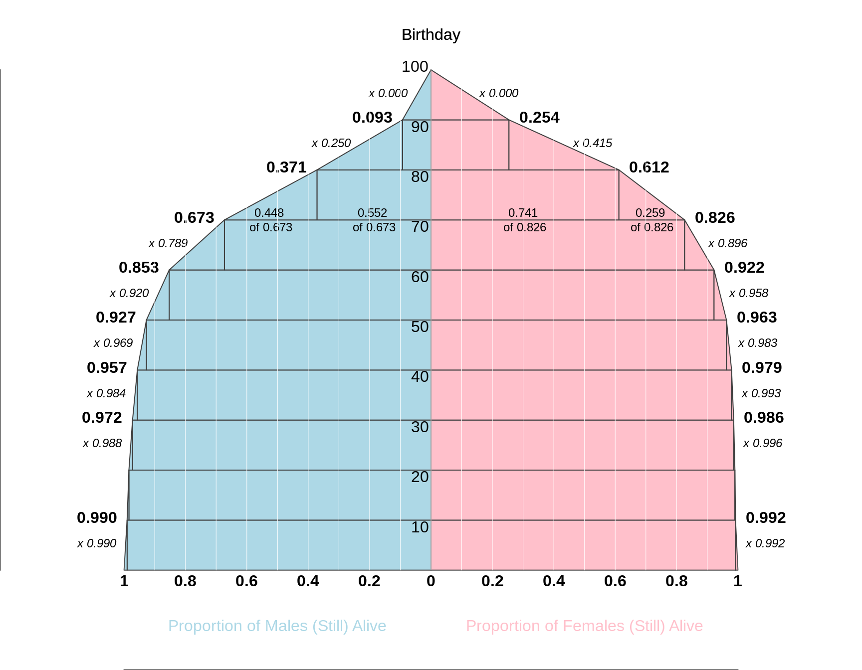
Figure 17.1: Life Tables based on abbreviated data from 1990 given in above table. The tabular orientation is 'bottom-up' rather than the conventional 'top-down' format, and side by side, in the spirit of population 'pyramids'. Also unusually, the 'survival surve' for males has the surviving proportion on the horizonatl axis, and the ages on the vertiacl axis. But if you were to rotate it by 90 degrees to the right, it would have conventional survival curve orentation.
For population pyramids, see https://www.populationpyramid.net/world/2019/
For dynamic ones, see https://www12.statcan.gc.ca/census-recensement/2016/dp-pd/pyramid/pyramid.cfm?geo1=01&type=1
17.2.3 Life Tables [2018]
For males and females separately, extract the 22 [conditional] probabilities of dying within the (1, 4 or 5 year) age intervals shown in Table 3.9 of this Institut de la statistique du Quebec report. They can be found in the \(q_x\) column [ x: age; q\(_x\) : given survival to birthday x, probability of dying between birthday x and birthday x+a, where a, a=1, 4 et 5.]
- Use these to compute the surviving fractions at each of the birthdays shown in Table 3.9. As a double check on your answers, you have the \(l_x\) columns in Table 3.9 [l\(_x\): number surviving at x-th birthday.] Hint: instead of using a loop, you can use the 'cumulative product' function
cumprod. For example,cumprod(c(0.9, 0.8, 0.7))yields the vector of length 3, namely 0.9, 0.9 \(\times\) 0.8 = 0.72, and 0.9 \(\times\) 0.8 \(\times\) 0.7 = 0.504. - Plot the fractions against the ages, overlaying one curve on the other. Make sure to label the axes appropriately, and using large enough lettering that people at the right hand of the age scale, where most of the action is, can read them.
- Visually measure the median survival for each gender.
- Do you think the mean survival (the life-expectancy at birth) is smaller or larger than the median? Explain your reasoning.
- The best way to be sure is to have and plot the frequency distributions of the ages at death. Using the same logic as in question 2, derive these frequencies, and plot them. Note that the first 2 age-bins are narrower than the others, so make wahtever adjustments are needed.
- Why don't these frequency distributions match those shown in Figure 3.5 of the report?
- Examine Figure 3.15 of the report, and explain why life expectancies calculated from single-calendar-year data can 'wobble' quite a bit from year to year.
17.2.4 A simplified epidemic
[from Mosteller and Rourke Book]
An infectious disease has a one-day infectious period, and after that day the person who contracts it is immune. Six hermits (numbered 1,2, 3, 4, 5, 6, or named A-F) live on an island, and if one has the disease he randomly visits another hermit for help during his infectious period. If the visited hermit has not had the disease, he catches it and is infectious the next day. Assume hermit 1 has the disease today, and the rest have not had it. In the pre-R era students were asked to throw a die to choose which hermit he visits (ignore face 1) Today you are asked to use the sample function in R to choose which hermit he visits. That hermit is infectious tomorrow. Then 'throw' (or use R) again to see which hermit he visits, and so on. Continue the process until a sick hermit visits an immune one and the disease dies out.
- Repeat the 'experiment' several times and find
- the average number who get the disease
the probability that (the proportion of experiments in which) everyone gets the disease.
Try to figure out a closed-form (algebraic) expression for the answer to the second part.
one.random.sequence =function(n.hermits=6){ # max 26, for 1-letter names
    names = LETTERS[1:n.hermits]
    who.is.infectious.today = 1
    trail = names[who.is.infectious.today]
    for(visit in (1:(n.hermits-1)) ) {
        who.infectious.hermit.visits =
         sample( (1:n.hermits)[-who.is.infectious.today], 1)
       trail = c(trail, names[who.infectious.hermit.visits])
    }
    return(trail)
}

(s = one.random.sequence(6)) ; duplicated(s)
## [1] "A" "F" "E" "E" "E" "B"## [1] FALSE FALSE FALSE TRUE TRUE FALSEN.SIMS = 100; n.hermits = 6
sequences = matrix(NA,N.SIMS,n.hermits)
for(i.row in 1:N.SIMS ){
sequences[i.row,1:6] = one.random.sequence(n.hermits)
}
first.duplicate = function(x){
d = duplicated(x)
result = length(x)+1
if(any(d)) result = min( (1:n.hermits)[duplicated(x)] )
return(result)
}
when.first.dup.happens = apply(sequences,1,first.duplicate)
table(when.first.dup.happens)## when.first.dup.happens
## 3 4 5 6 7
## 21 39 23 16 117.2.5 Screening for HIV
See Figure 1 'Meaning of Positive HIV Tests for HIV') in the article Can we afford the false positive rate?
Use
Rto redraw their FigureAdd on top of it a curve for a population with a 1% prevalence.
Add a curve for a prevalence of 0.16%, but assuming sensitivity is only 90%.
17.2.6 Duplicate Birthdays
[The exercises are found at the end of this sub-section]
For 13 years in the 607 course from 1981 to 1993, JH handed out a page with a 12 x 31 grid and asked the students to indicate their birthday (month and day). The numbers of students in the class ('n') varied from 19 to 52 (mean 32, median 33) The results, in 'raw' form here, may surprize you. In 10 of the 13 classes, there was at least one duplicate birthday.
By the way, the 'Birthday Problem' is a classic in probability classes.
year=c(0.8+(1981:1984),0.8+(1986:1988),
       1989.4,1989.8,0.4+(1990:1992),1993.8)
n = c(27,37,33,20,21,19,39,31,31,52,43,49,32)
at.least.one.duplicate.birthday =
   c(TRUE,TRUE,TRUE,FALSE,TRUE,FALSE,TRUE,TRUE,
     FALSE,TRUE,TRUE,TRUE,TRUE)
cbind(year,n,at.least.one.duplicate.birthday)
## year n at.least.one.duplicate.birthday
## [1,] 1981.8 27 1
## [2,] 1982.8 37 1
## [3,] 1983.8 33 1
## [4,] 1984.8 20 0
## [5,] 1986.8 21 1
## [6,] 1987.8 19 0
## [7,] 1988.8 39 1
## [8,] 1989.4 31 1
## [9,] 1989.8 31 0
## [10,] 1990.4 52 1
## [11,] 1991.4 43 1
## [12,] 1992.4 49 1
## [13,] 1993.8 32 1sum(at.least.one.duplicate.birthday)## [1] 10cat("n's in the classes without a duplicate:")## n's in the classes without a duplicate:n[!at.least.one.duplicate.birthday]## [1] 20 19 31Leaving out people born on Feb. 29, and assuming [FOR NOW] all of the 365 birthdays are equally likely, we have the following formula for the probability of NO duplicate birthday in a sample of \(n\). By subtracting this probability from 1 (a common 'trick' when working with the probability of 'at least' ... ), we obtain the probability of AT LEAST ONE duplicate birthday:
\[Prob[all \ n \ birthdays \ are \ different] = \frac{365}{365} \times \frac{364}{365} \times \frac{363}{365} \times \dots \times \frac{365-(n-1)}{365}.\]
Let's work this out (or tell R to work it out) for n's all the way from 1 to 365, and show the probabilities for the 13 classes, overlaid on all of the probabilities for \(n\) from 1 to 60.
prob.all.n.different = cumprod( (365:1) / rep(365,365) )

prob.all.different = round(prob.all.n.different[n],2)
prob.at.least.1.duplicate = 1 - prob.all.different

par(mfrow=c(1,1),mar = c(4.5,5,0,0))
plot(1:60,prob.all.n.different[1:60],type="l",
     cex.axis=1.25,cex.lab=1.25,
     xlab="n",col="blue",ylab="Probability")

abline(h=seq(0,1,0.1),col="lightblue")
abline(h=0.5,col="lightblue",lwd=2)
abline(v=seq(0,60,5),col="lightblue")

lines(1:60,1-prob.all.n.different[1:60],col="red")

points(n,prob.all.different,pch=19,cex=0.5)
points(n,1-prob.all.different,pch=19,cex=0.5)

points(n,at.least.one.duplicate.birthday,
       pch="X",cex=1.0,
       col=c("blue","red")[1+at.least.one.duplicate.birthday])

text(35,1-prob.all.n.different[35],
     "Prob. at least 1 duplicate",
     cex=1.5,col="red",adj=c(0,1.25))

text(35,prob.all.n.different[35],
     "Prob. all n are different",
     cex=1.5,col="blue",adj=c(0,-0.25))
Why is the probability so much higher than you would naively think?
If in a class of 30, we ask you what the probability is, you are likley to reason like this ...
'30 out of 365, so about 1 chance in 12 or so, or about 8%'.
BUT, by reasoning this way, you are just thinking about the probability that YOUR birthday will match the birthday of someone else. But then EVERYONE ELSE has to go through the same calculation, so there are a lot of possibilities for a match, between someone else and someone else.
An easy way to appreciate the large number opportunities there are for a match is to look at a random sample of 30 birthdays, and see if they contain a match. If you can't sort them first, you will have to compare the 2nd with the 1st (thats 1), the 3rd with the 1st and the 2nd (2 more), the 4rd with the 1st and the 2nd and 3rd (3 more), and so on, so 1 + 2+ ... + 29 = 435 in all! But if you are the first to call out your birth, and then look/listen for a match with YOUR birthday, thats just 29 others. So instead of 1/12, the probability of SOME match (anyone with anyone else) os a LOT higher than 1/12. (From the blue graph, it's about 70%!).
all.birthdays =
read.table(
   "http://www.biostat.mcgill.ca/hanley/statbook/BirthdayProbabilities.txt",
   as.is=TRUE)

# (as.is=TRUE doesn't convert alphabetic variables into factors)

plot(1:366,all.birthdays$prob,
      ylim=c(0,max(all.birthdays$prob)),
      cex = 0.5,pch=19,
      xlab="Days of Year (1=Jan 1, 366=Dec 31)")
abline(h= c(0, 1/(365:366)))
abline(v= seq(0,366,30),col="lightblue")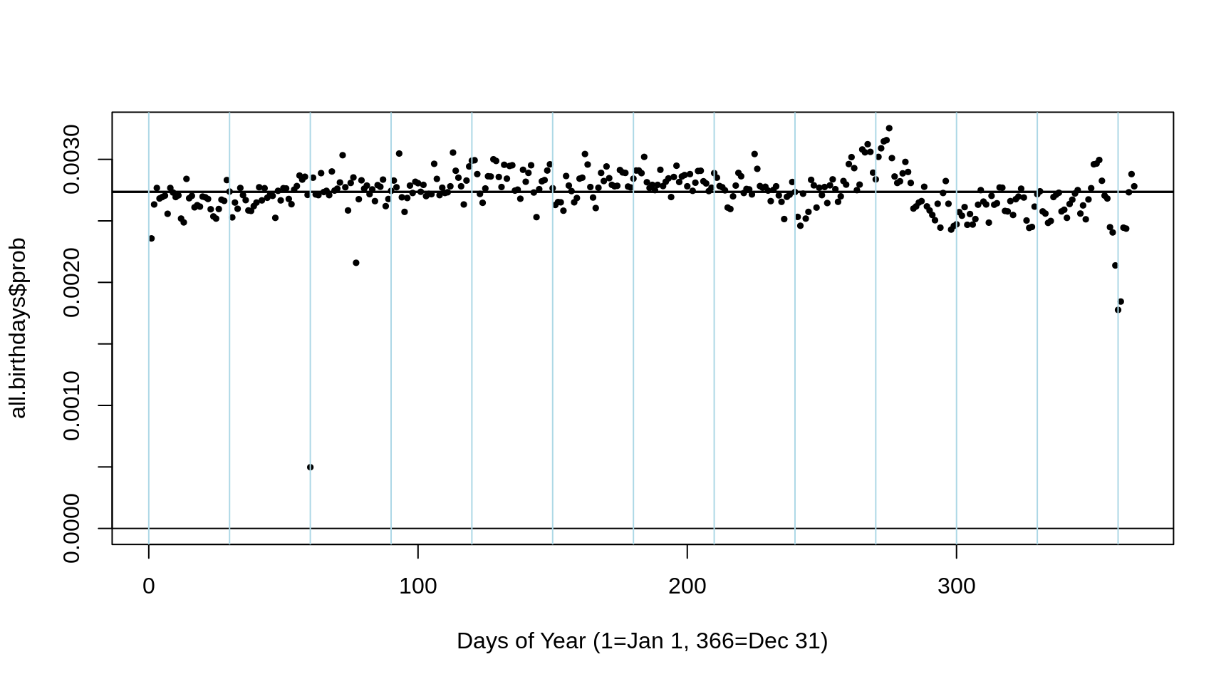
sample.of.30 = sample(all.birthdays$Birthday,30,replace=TRUE)

noquote(sample.of.30)
## [1] Jun 20 Mar 16 Mar 09 Oct 16 Jun 04 Mar 13 Oct 14 Nov 11 Feb 26 May 16
## [11] Feb 14 Jul 03 Jun 26 Apr 24 Jun 23 Sep 06 May 21 Nov 10 Jul 20 Apr 23
## [21] Oct 01 Mar 04 Jan 29 Dec 27 Aug 24 Jan 12 Aug 28 Aug 22 Oct 05 May 23If you have the software, you would sort this list first,
noquote( sort(sample.of.30) )## [1] Apr 23 Apr 24 Aug 22 Aug 24 Aug 28 Dec 27 Feb 14 Feb 26 Jan 12 Jan 29
## [11] Jul 03 Jul 20 Jun 04 Jun 20 Jun 23 Jun 26 Mar 04 Mar 09 Mar 13 Mar 16
## [21] May 16 May 21 May 23 Nov 10 Nov 11 Oct 01 Oct 05 Oct 14 Oct 16 Sep 06so its easier to spot any duplicates. And, if this is too laborious to do manually, you can use the unique and duplicated functions in R
unique.birthdays = unique(sample.of.30)
( n.unique = length(unique.birthdays) )
## [1] 30duplicated(sample.of.30)## [1] FALSE FALSE FALSE FALSE FALSE FALSE FALSE FALSE FALSE FALSE FALSE FALSE
## [13] FALSE FALSE FALSE FALSE FALSE FALSE FALSE FALSE FALSE FALSE FALSE FALSE
## [25] FALSE FALSE FALSE FALSE FALSE FALSE( sample.of.30[ duplicated(sample.of.30) ] )## character(0)But, as computer science people will tell you, sorting large lists takes a lot of computing. Just think about how you would manually sort a list of 1 million or 1 billion! The book Algorithms to Live By explains this well.
In the early 1980s, Loto Quebec did not realize that there is a high chance of duplicates when the sample size is sizeable, and, as we tell in our case III, they were embarrassed. We tell more of the story here. They now SORT the list first, to find duplicates.
Exercises
- By splitting 4 successive nodes into FirstDuplicate = YES or NO, draw a probability tree for the first 4 birthdays announced (Such a tree, with each node splitting into an Infected hermit visit a Susceptible hermit or visit an immune/recovered hermit, can help you think through the simulated mini-epidemic. BTW: you hear a lot abot SIR models thse days, and you will have seen the 'R' category displated in many of the covid-19 epidemic graphs)
- Using the
prob.all.n.differentvector derived above, calculate, by successive subtractions^ or otherwise, the probability that the first duplicate will show up on the [\(Y\) =] 2nd, 3rd, ... birthday announced. Plot the frequency distribution of \(Y\). - By simulation, estimate the probability that 'in 20 draws one will not obtain a duplicate' ^^.
- In every class where this Birthday Problem is addressed, students object that leaving out Feb 29 and assuming all of the 365 birthdays are equally likely are not realistic. Births vary somewhat by season and more so by day of the week So, in reality, are the probabilities of at least one duplicate birthday higher or lower than you have calculated above? Or is it impossible to say in which direction they are moved?
To investigate this use theall.birthdaysdataset created in theRcode above. you can visualize the variation in the 366 probabilites by using this statementplot(1:366,all.birthdays$prob, ylim=c(0,max(all.birthdays$prob)), cex = 0.5,pch=19, xlab="Days of Year (1=Jan 1, 366=Dec 31)")and drawing grids with these onesabline(h= c(0, 1/(365:366)))andabline(v= seq(0,366,30),col="lightblue").
This distribution is based on all births in a certain country from 1990-1999 [the years when many of you were born]. From it, draw several samples of 20 birthdays, and calculate the proportion of these sets in which the 20 birthdays are unique, and conversely, contain at least 1 duplicate. SomeRcode is given below. - Try to figure out from the features of the plot what country the birthday data are from? Explain your reasoning.
- Just from how much the 366 probabilities 'wobble' around 1/365 or 1/366, try to figure out (approximately, to within an order of magnitude) how many births were used to derive the 366 proportions. For example, is it a country with a population size such as China, India, USA, Germany, New Zealand, Iceland, Prince Edward Island, the Yukon Territory, etc?
https://rss.onlinelibrary.wiley.com/doi/full/10.1111/j.1740-9713.2013.00705.x
^ If \(Y\) = which draw produces 1st duplicate (so \(Y\) = 2,... 365). e.g.
Pr[$Y$ > 6] = Pr[Y = 7 or 8 or 9 or .. or 365 ]
Pr[$Y$ > 7] = Pr[Y = .... 8 or 9 or .. or 365 ]
Difference: = Pr[Y = 7]
N.SIMS=100
n = 23
#PROBS = rep(1/366,366)    # ON  for comparison
PROBS  = all.birthdays$prob # OFF for comparison
B = matrix(
      sample(all.birthdays$Birthday,
             size = N.SIMS*n,
             prob = PROBS,
             replace=TRUE),
      nrow = N.SIMS,  ncol = n)
head(B,2)
## [,1] [,2] [,3] [,4] [,5] [,6] [,7] [,8]
## [1,] "Feb 09" "Jul 09" "Apr 02" "Sep 17" "Nov 27" "Oct 28" "Oct 16" "May 25"
## [2,] "Jul 17" "Mar 21" "Nov 29" "Jun 20" "Apr 03" "Dec 13" "Jan 18" "Jun 04"
## [,9] [,10] [,11] [,12] [,13] [,14] [,15] [,16]
## [1,] "Feb 28" "Apr 24" "Nov 21" "Jun 05" "Jun 20" "Feb 08" "Jun 03" "Nov 30"
## [2,] "Jan 13" "Aug 21" "Feb 08" "Dec 06" "Aug 12" "Dec 06" "Nov 11" "May 10"
## [,17] [,18] [,19] [,20] [,21] [,22] [,23]
## [1,] "Jul 31" "Sep 18" "Oct 20" "May 16" "May 22" "Jan 02" "Nov 26"
## [2,] "Aug 07" "Nov 11" "Dec 14" "Dec 23" "Jul 28" "Oct 24" "Feb 13"duplicate = apply(B,1,
function(x) sum(duplicated(x)) > 0 )
noquote(paste(sum(duplicate), "duplicates /",
N.SIMS,
" ; larger N.SIMS: more precise probability estimate.",collapse=" "))## [1] 52 duplicates / 100 ; larger N.SIMS: more precise probability estimate.17.2.7 Chevalier de Méré
[see here}(https://www.cut-the-knot.org/Probability/ChevalierDeMere.shtml) or
Gamblers in 17th century France used to bet on the event of getting at least one 1 'six' in four rolls of a die or in 1 roll of 4 dice [dice is plural for die]. As a more trying variation, two dice were rolled 24 times with a bet on having at least one double six. Chevalier de Méré who expected a couple of sixes to turn up in 24 double rolls with the frequency of a six in 4 single rolls. However, he lost consistently.
Simulate a large number of each of these games, and estimate the probability of getting (a) at least one six in four rolls of a dice (b) at least one "double six" when a pair of dice is thrown 24 times
Why does it take a large number of simulations to determine which game offers the better chance of winning?
Can you work out the probabilities directly?
https://www.casino-games-online.biz/dice/chevalier-de-mere.html
17.3 Other Exercises (under construction)
17.3.1 HIV transmission
[ probability per act ]
Napoleon
Minard http://euclid.psych.yorku.ca/www/psy6135/tutorials/Minard.html
Efron Monty Hall
The Economist
Wald : CF screening
OJ p-value
Adult soccer ball.. wrong probability
Vietnam deaths
NHL birthdays
Buffon's needle
Estimating Pi
Similar
Adult size soccer ball
Medical School admission rates, by gender.
Vietnam war deaths, by month of birth
NHL success, by month of birth
John Snow, cholera deaths South London, by source of drinking water
Galton
Greenwood
Mosteller
Ages of books
ngrams
- Prob of
- duplicate birthdays in a sample of \(n\) persons
- surviving from 80th to 85th birthday if the (conditional) 1-year at a time proportions dying (risks) are ...
- Chevalier de Méré no 6, at least 1 six.
- Variation with and without constraints
-3- "Duplicate Numbers" [mini-version of birthday problem] To appreciate the high probability of duplicate birthdays, take a simpler case of drawing single digit numbers at random from a Random Number Table or spreadsheet until one gets a duplicate. (also, try actually doing it to see how many draws it takes) a Calculate the probability that in 5 draws one will not obtain a duplicate, i.e., the probability of a sequence 1st# ; 2nd# [≠ 1st#] 3rd# [≠ 2nd# ≠ 1st#] 4th# [≠ 3rd# ≠ 2nd# ≠ 1st#] 5th# [≠ 4th# ≠3rd# ≠ 2nd# ≠ 1st#] b Calculate, by successive subtractions* or otherwise, the probability that the first duplicate will show up on the [Y =] 2nd, 3rd, ...11th draw. Plot the frequency distribution of the # draws, Y, until a duplicate.
Ice Breakup Dates
Here are some details on the Nenana Ice Classic More here
17.3.2 The 2018 Book of Guesses
We are keen to establish the distribution of guesses, with the guessed times measured from midnight on December 31, 2017. Thus a guess of April 06, at 5:15 p.m. would be measured as 31 + 28 + 31 + 5 + 12/24 + (5+ 15/60)/24 = 95.71875 days into the year 2018.
It would be tedious to apply optical character recognition (OCR) to each of the 1210 pages in order to be able to computerize all 240,000 guesses. Instead, you are asked to reconstruct the distribution of the guesses in two more economical ways:
By determining, for (the beginning of) each day, from April 01 to June 01 inclusive, the proportion, p, of guesses that predede that date. [ In
R, if p = 39.6% of the guesses were below 110 days, we would write this as pGuessDistribution(110) = 0.396. Thus, if we were dealing with the location of a value in a Gaussian ('normal') distribution, we would writepnorm(q=110, mean = , sd = )] Once you have determined them, plot these 62 p's (on the vertical axis) against the numbers of elapsed days (90-152) on the horizontal axis.By determining the 1st, 2nd, ... , 98th, 99th percentiles. These are specific examples of 'quantiles', or q's. The q-th quantile is the value (here the elapsed number of days since the beginning of 2018) such that a proportion q of all values are below this value, and 1-q are above it. [ In
R, if 40% of the guesses were below 110.2 days, we would write this as qGuessDistribution(p=0.4) = 110.2 days. Thus, if we were dealing with the 40th percentile of a Gaussian distribution with mean 130 and standard deviation 15, we would writeqnorm(p=0.4, mean = 130, sd = 15). ] Once you have determined them, plot the 99 p's (on the vertical axis) against the 99 (elapsed) times on the horizontal axis.Compare the Q\(_{25}\), Q\(_{50}\), and Q\(_{75}\) obtained directly with the ones obtained by interpolation of the curve showing the results of the other method.
Compare the directly-obtained proportions of guesses that are before April 15, April 30, and May 15 with the ones obtained by interpolation of the curve showing the results of the other method.
By successive subtractions, calculate the numbers of guesses in each 1-day bin, and make a histogram of them. From them, calculate the mean, the mode, and the standard deviation.
To measure the spread of guesses, Galton, in his vox populi (wisdom of crowds) article, began with the interquartile range (IQR), i.e. the distance between Q75 and Q25, the 3rd and 1st quartiles. In any distribution, 1/2 the values are within what was called the 'probable error (PE) of the mean; i.e., it is equally probable that a randomly selected value would be inside or outside this middle-50 interval. Today, we use standard deviation (SD) instead of probable error. In a Gaussian distribution, some 68% of values are within 1 SD of the mean, whereas 50% of values are within 1 PE of the mean. We can use R to figure out how big a PE is in a Gaussian distribution compared with a SD. By setting the SD to 1, and the eman to 0, we have
Q75 = qnorm(p = 0.75, mean=0, sd=1)
round(Q75,2)
## [1] 0.67i.e, a PE is roughtly 2/3rds of a SD.
Galton -- convert to SD.
Geometric mean Amsterdam study
How far off was the median guess in 2018 from the actual time? Answer in days, and (with reservations stated) as a percentage?
Why did the experts at the country fair do so much better?
Where were the punters in 2019 wrt the actual ?
https://www.all-about-psychology.com/the-wisdom-of-crowds.html
http://galton.org/essays/1900-1911/galton-1907-vox-populi.pdf
[Nenana Ice Classic]
Tanana River
17.3.3 Trends over the last 100 years
fill in the data since 200x.
cbind with ...
time trends
morning vs afternoon ?
2019 extreme... how many SD's from the line?
- Where were the punters in 2019 wrt the actual ?
Sources:
1917-2003 data in textfile on course website;
http://www.nenanaakiceclassic.com/ for data past 2003
ascii (txt) and excel files with data to 2003
Working in teams of two ...
*Create a dataframe containing the breakup data for the years 1917-2007. Possible ways to do so include: directly from the ascii (txt) file; from the Excel file
*From the decimal portion of the Julian time, use R to create a frequency table of the hour of the day at which the breakup occurred.
*From the month and day, use R to calculate your own version of the Julian day (and the decimal portion if you want to go further and use the hour and minute)
*Is there visual evidence that over the last 91 years, the breakup is occurring at an earlier date?
*Extract the date and ice thickness measurements for the years 1989-2007 from the website and use (your software of choice) R to create a single dataset with the 3 variable, year, day and thickness. From this, fit a separate trendline for each year, and calculate the variability of these within-year slopes.
- Galton’s data on family heights
These data were gathered to examine the relation between heights of parents and heights of their (adult) children. They have been recently 'uncovered' from the Galton archives. As a first issue, for this exercise, you are also asked to see whether the parent data suggest that stature plays "a sensible part in marriage selection”.
For the purposes of this exercise, the parent data [see http://www.epi.mcgill.ca/hanley/galton ] are in a file called parents.txt , with families numbered 1-135, 136A, 136-204 ( {the heights of the adult offspring will be used in a future exercise)
Do the following tasks using R
Categorize each father's height into one of 3 bins (shortest 1/4, middle 1/2, tallest 1/4). Do likewise for mothers. Then, as Galton did [ Table III ], obtain the 2-way frequency distribution and assess whether "we may regard the married folk as picked out of the general population at haphazard".
Calculate the variance Var[F] and Var[M] of the fathers' [F] and mothers' [M] heights respectively. Then create a new variable consisting of the sum of F and M, and calculate Var[F+M]. Comment. Galton called this a "shrewder" test than the "ruder" one he used in 1.
When Galton first anayzed these data in 1885-1886, Galton and Pearson hadn't yet invented the correlation coefficient. Calculate this coefficient and see how it compares with your impressions in 1 and 2.
- Temperature perceptions
Create 5 datasets from the questionnaire data on temperature perceptions etc.
by importing directly from the Excel file applied to .csv version of Excel file);
by first removing the first row (of variable names) and exporting the Excel file into a 'comma-separated-values" (.csv) text file, then ...
reading the data in this .csv file via the INFILE and INPUT statements in a SAS DATA step,
[SAS] INFILE 'path' DELIMITER =","; INPUT ID MALE $ MD $ EXAM TEMPOUTC TEMPINC TEMPOUTF TEMPINF TEMPFEEL TIME PLACE $ ;
- by reading the data in the text file temps_1.txt into
the SAS dataset via the INFILE and INPUT statements. Notice that the 'missing' values use the SAS representation (.) for missing values.
or the Stata dataset using the 'infile' command
- by reading the data in the text file temps_2.txt via [in SAS] the INFILE and INPUT statements in a DATA step or [in Stata] the 'infix' command.
Here you will need to be careful, since 'free-format' will not work correctly (it is worth trying free format with this file, just to see what goes wrong!). When using the INFILE method, you can control some of the damage by using the 'MISSOVER' option in the INFILE statement: this keeps the INPUT statement from continuing on into the next data line in order to find the (in our example) 11 values implied by the variable list. JH uses this 'defensive' option in ALL of his INFILE statements.
- by cutting and pasting the contents of the text file temps_2.txt directly into the SAS or Stata program - in SASthe lines of data go immediately after the DATALINES statement, and there needs to be a line containing a semicolon to indicate the end of the data stream. In Stata, the lines of data go immediately after the infile or infix statement, and there needs to be a line containing the word 'end' to indicate the end of the data stream
This Cut and Paste Method is NOT RECOMMENDED when the number of observations is large, as it is too all too easy to inadvertently alter the data, and the SAS/Stata porogram becomes quite long and unwieldy. It is Good Data Management Practice to separate the program statements from the data.
[Run [in SAS] PROC MEANS [in Stata] the 'describe' command, on the numerical variables, and [in SAS] PROC FREQ or [in Stata] the 'tabulate' command, on the non-numerical variables, to check that the 5 datasets you created contain the same information. Also, get in the habit of viewing or printing several observations and checking the entries against the 'source'.
When using (i), have SAS show you the SAS statements generated by the wizard. Store these, and the DATA steps for (ii) to (v) in a single SAS program file (with suffix .sas).
Annotate liberally using comments:
in SAS, either begin with * ; or enclose with /* ... */
in Stata ..begin the line with * or place the comment between /* and */ delimiters or begin the comment with // or begin the comment with ///
Q2
Use one of these 5 datasets, and the appropriate [in SAS, PROCs (see Exploring Data under UCLA SAS Class Notes 2.0)], or [in Stata, the list comamnd, and the analyses from the Statistics menu] tolist the names and characteristics of the variables
list the first 5 observations in the dataset
list the id # and the responses just to q3, w5 and q6, for all respondents, with respondents in the order: female MDs, male MDs, female non-MDs, male non-MDs. Indicate the [sub-]statement that is required to reverse this order.
create a 2-way frequency table, showing the frequencies of respondents in each of the 2 (MD nonMD) x 2 (male female) = 4 'cells' (one defintion of an epidemiologist is 'an MD broken down by age and sex'). Turn off all the extra printed output, so that the table just has the cell frequencies and the row and column totals.
compare the mean and median attitude to exams in MDs vs. non-MDs (hint: in SAS, the CLASS statement may help). Get SAS/Stata to limit the output to just the 'n', the min, the max, the mean and the median for each subgroup. And try to also get it to limit the number of decimal places of output (in SAS the MAXDEC option is implememnted in some procedures, but as far as JH can determine not in all)
compare the mean temperature perceptions (q6) of male and female respondents
[in SAS] create a low-res ('typewriter' resolution) scatterplot of the responses to q5 (vertical axis) vs. q4 (horizonatal axis), using a plotting symbol that shows whether the responsdent is a male or a female. If we have not covered how to show this '3rd dimension', look at the ONLINE Documentation file {the guide for most of the procedures covered in this set of exercises is in the Base SAS Procedures Guide; other procedures are in sthe more advanced 'STAT' module}. You can specify the variable whose values are to mark each point on the plot. See PLOT statement in PROC PLOT, and the example with variables height weight and gender. [in Stata] use the (automatically hi-res) graphics capabilities available from the 'Graphics' menu
[if SAS] Put all of the programs for Q1, and all of these program steps and output for Q2 in a single .txt file (JH will use a mono-spaced font such as Courier to view it -- that way the alignment should be OK), with PROC statements interleaved with output, and a helpful 2-line title (produced by SAS, but to your specifications) over top of each output. Get SAS to set up the output so that there are no more that 65 horizontal characters per line (that way, lines won't wrap-around when JH views the material).
[if Stata] paste the results and graphics into Word.
NOTE: To be fair to SAS, it CAN produce decent (and even some publication-quality) graphics. See http://www.ats.ucla.edu/stat/sas/topics/graphics.htm
Then submit the text file electronically (i.e., by email) to JH by 9 am on Monday October 2.
- Natural history of prostate cancer
Q1
The following data items are from an investigation into the natural history of (untreated) prostate cancer [ report (.pdf) by Albertsen Hanley Gleason and Barry in JAMA in September 1998 ].
id, dates of birth and diagnosis, Gleason score, date of last contact, status (1=dead, 0=alive), and -- if dead -- cause of death (see 2b below). data file (.txt) for a random 1/2 of the 767 patients
Compute the distribution of age at diagnosis (5-year intervals) and year of diagnosis (5 year intervals). Also compute the mean and median ages at diagnosis.
For each of the 20 cells in Table 2 (5 Gleason score categories x 4 age-at-dx categories), compute the
number of man-years (M-Y) of observation
number of deaths from prostate cancer(1), other causes(2), unknown causes(3)
prostate cancer(1) death rate [ deaths per 100 M-Y ]
proportion who survived at least 15 years.
For a and b you can use the 'sum' option in PROC means; ie PROC MEANS data = ... SUM; VAR vars you want to sum; BY the 2 variables that form the cross-classification. Also think of a count as a sum of 0s and 1s. For c (to avoid having to compute 20 rates by hand), you can 'pipe' i.e. re-direct the sums to a new sas datafile, where you can then divide one by other to get (20) rates. Use OUTPUT OUT = .... SUM= ...names for two sums;
On a single graph, plot the 5 Kaplan-Meier survival curves, one for each of the 5 Gleason score categories (PROC LIFETEST .. Online help is under the SAS STAT module, or see http://www.ats.ucla.edu/stat/sas/seminars/sas_survival/default.htm. For Stata, see http://www.ats.ucla.edu/stat/stata/seminars/stata_survival/default.htm.
[OPTIONAL] In order to compare the death rates with those of U.S. men of the same age, for each combination of calendar year period (1970-1974, 1975-1979, ..., 1994-1999) and 5 year age-interval (55-59, 60-64, ... obtain
the number of man-years of follow-up and
the number of deaths.
Do so by creating, from the record for each man, as many separate observations as the number of 5yr x 5yr "squares" that the man traverses diagonally through the Lexis diagram [ use the OUTPUT statement within the DATA step]. Then use PROC MEANS to aggregate the M-Y and deaths in each square. If you get stuck, here is some SAS code that does this, or see the algorithm given in Breslow and Day, Volume II, page ___
Put all of the program steps and output into a single .txt file. JH will use a mono-spaced font such as Courier to view it -- that way the alignment should be ok. Interleave DATA and PROC statements with output and conclusions, and use helpful titles (produced by SAS, but to your specifications) over top of each output. Get SAS to set up the output so that there are no more that 65 horizontal characters per line -- that way, lines won't wrap-around even when the font used to view your file is increased. Show relevant excerpts rather than entire listings of datafiles. Annotate liberally. Submit the text file electronically (i.e., by email) to JH by 9 am on Monday Nov 7.
- Serial PSA values
Q1
These two files contain PSA values [pre-] and [post-] treatment of prostate cancer *.
- Create a 'wide' PSA file of 25 log-base-2 PSA values per man (some will be missing, if PSA not measured 25 times). Print some excerpts.
(b)From the dataset created in (a), create a long file, with just the observations containing the non-missing log-base-2 PSA values [OUTPUT statement in DATA step]. Print and plot some excerpts.
- From the dataset created in (b), create a wide file [ RETAIN, first. and last. helpful here; or use PROC TRANSPOSE ]. Print some excerpts.
- The order of the variables is given in this sas program . Some of the code in the program may also be of help.
Put all of the program steps and output into a single .txt file. JH will use a mono-spaced font such as Courier to view it -- that way the alignment should be ok. Interleave DATA and PROC statements with output and conclusions, and use helpful titles (produced by SAS, but to your specifications) over top of each output. Get SAS to set up the output so that there are no more that 65 horizontal characters per line -- that way, lines won't wrap-around even when the font used to view your file is increased. Show relevant excerpts rather than entire listings of datafiles. Annotate liberally. Submit the text file electronically (i.e., by email) to JH by 9 am on Monday Nov 14.
- Graphics
1a
Re-produce (or if you think you can, improve on) three of the graphs shown in "Examples of graphs from Medical Journals." These examples are in a pdf file on the main page. Use Excel for at least one of them, and R/Stata/SAS for at least one other. Do not go to extraordinary lengths to make them exactly like those shown -- the authors, or the journals themselves, may have used more specialized graphics software. You may wish to annotate them by making (and sharing with us) notes on those steps/options that were not immediately obvious and that took you some effort to figure out. Insert all three into a single electronic document.
1b
Browse some medical and epidemiologic journals and some magazines and newspapers published in the last 12 months, Identify the statistical graph you think is the worst, and the one you think is the best. Tell us how many graphs you looked at, and why you chose the two you did. If you find a helpful online guide or textbook on how to make good statistical graphs, please share the reference with us. [The bios601 site http://www.epi.mcgill.ca/hanley/bios601/DescriptiveStatistics/ has a link to the Textbook by Cleveland and the book "R Graphics" by Paul Murrell.
If possible, electronically paste the graphs into the same electronic file you are using for 1a.
2
[OPTIONAL] The main page has a link to a lifetable workbook containing three sheets. Note that the 'lifetable' sheet in this workbook is used to calculate an abridged current life table based on the 1960 U.S. data. Use this sheet as a guideline, and create a current life-table ('complete', i.e., with 1-year age-intervals) for Canadian males, using the male population sizes, and numbers of deaths, by age, Canada 2001. [The calculations in columns O to W of the lifetable sheet are not relevant for this exercise]. Details on the elements of, and the construction of current lifetables can be found in the chapters (on website) from the textbooks by Bradford Hill and Selvin, and in the technical notes provided by the US National Center for Health Statistics in connection with US Lifetable 2000. See also the FAQ for 613 from 2005. The fact that the template is for an abridged life table, with mostly 5-year intervals, whereas the task is to construct a full lifetable with 1 year intervals, caused some people problems last year.. they realized something was wrong when the life expectancy values were way off!
Since this is an exercise, and not a calculation for an insurance company that wants to have 4 sig. decimal places, don't overly fuss about what values of 'a' you use for the early years.. they don't influence the calculations THAT much: If you try different sets of values (such as 0.1 in first year and 0.5 thereafter) you will not find a big impact. But don't take my word for it .. the beauty of a spreadsheet is that you can quickly see the consequences of different assumptions or 'what ifs'.
[In practice, in order not to be unduly influenced by mortality rates in a single calendar year (e.g. one that had a very bad influenza season), current lifetables are usually based on several years of mortality data. Otherwise, or if they are based on a small population, the quantities derived from them will exhibit considerable random fluctuations from year to year ]
Once you have completed the table, use the charting facilities in Excel to plot the survival curve for the hypothetical (fictitious) male 'cohort' represented by the current lifetable.
On a separate graph, use two histograms to show the distributions of the ages at death (i) for this hypothetical male 'cohort' and (ii) those males who died in 2001. To make it easy to compare them, superimpose the histograms or put them 'side by side' or 'back to back' within the same graph. Explain why the two differ in shape and location. Calculate/derive (and include them somewhere on the spreadsheet) the median and mean age at death in the hypothetical cohort and the corresponding statistics for the actual deaths in 2001.
- Possible Body Mass Indices
This exercise investigates different definitions of Body Mass Index (BMI).
BACKGROUND: With weight measured in Kilograms, and height in metres, BMI is usually defined as weight divided by the SQUARE of height, i.e., BMI = Wt / (Height*Height), or BMI = Wt/(height2) using, as SAS and several other programming languages do, the symbol for 'raised to the power of'. [ NB: Excel uses ^ to denote this ]
What's special about the power of 2? Why not a power of 1 i.e., Weight/height?
Why not 3, i.e., Weight/*(height3) ? Why not 2.5 i.e. Weight/(height2.5)?
One of the statistical aims of a transformation of weight and height to BMI is that BMI be statistically less correlated with height, thereby separating height and height into two more useful components height and BMI. For example in predicting lung function (e.g. FEV1), it makes more sense to use height and BMI than height and weight, since weight has 2 components in it -- it is partly height and partly BMI. Presumably, one would choose the power which minimizes the correlation.
The task in this project is to investigate the influence of the power of height used in the ratio, and to see if the pattern of correlations with power is stable over different settings (datasets).
DATA: To do this, use 2 of the 6 datasets on the 678 webpage: [usernane is c678 and p w is H**J44 ]
- Children aged 11-16 Alberta 1985 (under 'Datasets')
- 18 year olds in Berkeley longitudinal study, born 1928/29 (under 'Datasets')
- Dataset on bodyfat -- 252 men (see documentation) (under 'Datasets')
- Pulse Rates before and after Exercise -- Australian undergraduates in 1990's (under 'Projects')
- Miss America dataset 1921-2000 (under 'Resources')
- Playboy dataset 1929-2000 (under 'Resources')
METHODS: First create each of the two SAS datasets, and if height and weight are not already in metres and Kg, convert them to these units. Drop any irrelevant variables. Inside each dataset, create a variable giving the source of the data (we will merge the two -- and eventually all six-- datasets, so we need to be able to tell which one each observation came from).
Combine the two datasets, i.e. 'stack' them one above the other in a single dataset. Print out some excerpts.
For each subject in the combined dataset, create 5 versions of <
Calculate the correlation between the 'BMI' obtained with each of these powers, and height. Do this separately for the observations from the two different sources (the BY statement should help here).
Report your CONCLUSIONS.
- Galton
The objective of this exercise is to examine the relation between heights of parents and heights of their (adult) children, using recently 'uncovered' data from the Galton archives, You are asked to assess if Galton's way of dealing with the fact that heights of males and females are quite different produces sharper correlations than we would obtain using 'modern' methods of dealing with this fact. As side issues, you are also asked to see whether the data suggest that stature plays "a sensible part in marriage selection" and to comment on the correlations of the heights in the 4 {father,son}, {father,daughter}, {mother,son} and {mother,daughter} pairings.
BACKGROUND: Galton 'transmuted' female heights into their 'male-equivalents' by multiplying them by 1.08, and then using a single combined 'uni-sex' dataset of 900-something offspring and their parents. While some modern-day anayysts would simply calculate separate correlations for the male and female offspring (and then average the two correlations, as in a meta-analysis), most would use the combined dataset but 'partial out' the male-females differences using a multivariable analysis procedure. The various multivariable procedures in effect create a unisex dataset by adding a fixed number of inches to each female's height (or, equivalently, in the words of one of our female PhD students, by 'cutting the men down to size'). JH was impressed by the more elegant 'proportional scaling' in the 'multiplicative model' used by Galton, compared with the 'just use the additive models most readiliy available in the software' attitude that is common today. In 2001, he located the raw (untransmuted) data that allows us to compare the two approaches.
DATA: For the purposes of this exercise, the data [see http://www.epi.mcgill.ca/hanley/galton ] are in two separate files:
- the heights# of 205 sets of parents ( parents.txt ) with families numbered 1-135, 136A, 136-204
the heights# of their 900-something* children ( offspring.txt ) with families numbered as above
The data on eight families are deliberately omitted, to entice the scholar in you to get into the habit of looking at (and even double checking) the original data. Since here we are more interested in the computing part in this course, and because time is short, ignore this invitation to inspect the data -- we already had a look at them in class. In practice, we often add in 'missing data' later, as there are always some problem cases, or lab tests that have to be repeated, or values that need to be checked, or subjects who didn't get measured at the same time as others etc.. JH's habit is to make the additions in the 'source' file (.txt or .xls or whatever) and re-run the entire SAS DATA step(s) to create the updated SAS dataset (temporary or permanent). If the existing SAS datset is already large, and took a lot of time to create, you might consider creating a small dataset with the new observations, and then stacking (using SE) the new one under the existing one -- in a new file. SAS has fancier ways too, and others may do things differently!
If your connection is too slow to view the photo of the first page of the Notebook, the title reads
FAMILY HEIGHTS (add 60 inches to every entry in the Table)
METHODS/RESULTS/COMMENTS:
Categorize each father's height into one of 3 subgroups (shortest 1/4, middle 1/2, tallest 1/4). Do likewise for mothers. Then, as Galton did [ Table III ], obtain the 2-way frequency distribution and assess whether "we may regard the married fold as picked out of the general population at haphazard".
Calculate the variance Var[F] and Var[M] of the fathers' [F] and mothers' [M] heights respectively. Then create a new variable consisting of the sum of F and M, and calculate Var[F+M]. Comment. Galton called this a "shrewder" test than the "ruder" one he used in 1. ( statistic-keyword VAR in PROC MEANS)
When Galton first anayzed these data in 1885-1886, Galton and Pearson hadn't yet invented the CORRelation coefficient. Calculate this coefficient and see how it compares with your impressions in 1 and 2.
Create two versions of the transmuted mother's heights, one using Galton's and one using the modern-day (lazy-person's, blackbox?) additive scaling [for the latter, use the observed difference in the average heights of fathers and mothers, which you can get by e.g., running PROC MEANS on the offspring dataset, either BY gender, or using gender as a CLASS variable]. In which version of the transmuted mothers' heights is their SD more simlar to the SD of the fathers? ( statistic-keyword STD in PROC MEANS)
Create the two corresponding versions of what Galton called the 'mid-parent' (ie the average of the height of the father and the height of the transmuted mother). Take mid-point to mean the half-way point (so in this case the average of the two)
Create the corresponding two versions (additive and multiplicative scaling) of the offspring heights (note than sons' heights remain 'as is'). Address again, but now for daughters vs sons, the question raised at the end of 4.
Merge the parental and offspring datasets created in steps 4 and 6, taking care to have the correct parents matched with each offspring (this is called a 1:many merge).
Using the versions based on 1.08, round the offspring and mid-parent heighs to the nearest inch (or use the FLOOR function to just keep the integer part of the mid-parent height --you need not be as fussy as Galton was about the groupings of the mid-parent heights), and obtain a 2-way frequency distribution similar to that obtained by Galton [ Table I ]. Note that, opposite to we might do today, Galton put the parents on the vertical, and the offspring on the horizontal axis. ( The MOD INT FLOOR CEIL and ROUND functions can help you map observations into 'bins' ; we will later see a way to do so using loops)
Galton called the offspring in the same row of his table a 'filial array'. Find the median height for each filial array, and plot it, as Galton did, against the midpoint of the interval containing their midparent -- you should have one datapoint for each array. Put the mid-parent values on the vertical, and the offspring on the horizontal axis. By eye, estimate the slope of the line of best fit to the datapoints. Mark your fitted line by 'manually' inserting two markers at the opposite corners of the plot. Does the slope of your fitted line agree with Galton's summary of the degree of "regression to mediocrity"? [ Plate IX ] Note that Galton used datapoints for just 9 filial arrays, choosing to omit those in the bottom and top rows (those with the very shortest and the very tallest parents) because the data in these arrays were sparse. ( By using the binned parental height in the CLASS statement in PROC MEANS or PROC UNIVARIATE, directing the output to a new SAS dataset, and applying PROC PLOT to this new dataset, you can avoid having to do the plotting manually See more on this in the FAQ)
Plot the individual unisex offspring heights (daughters additively transmuted) versus the mid-parent height (mothers transmuted). OVERLAY on it, with a different plotting symbol, the corresponding plot involving the multiplicatively transmuted offspring values (on the parent-axis, stay with Galton's definition of a midparent). (see FAQ) Compare the two, and have a look at Galton's fitted ellipse, corresponding to a bivariate normal distribution [ Plate X ]) {here, again, we would be more likely to plot the parents' heights on the horizontal, and the offspring heights on the vertical axis}.
For each of the following 'offspring vs. mid-parent' correlations, use the 'mid-parent' obtained using Galton's multiplicative method. Calculate (a) the 2 correlations for the 2 unisex versions of the offspring data (b) the sex-specific correlations (i.e., daughters and sons separately) and (c) the single parent-offspring correlation, based on all offspring combined, and their untransmuted heights, ignoring the sex of the offspring. Comment on the correlations obtained, and on the instances where there are big disparities between them. [ a PLOT, with separate plotting symbols for sons and daughters, might help in the case of (c) ]
Calculate the 4 correlations (i) father,son (ii) father,daughter, (iii) mother,son and (iv) mother,daughter. Comment on the pattern, and on why you think it turned out this way.
Put all of the program steps and output into a single .txt file. JH will use a mono-spaced font such as Courier to view it -- that way the alignment should be ok. Interleave DATA and PROC statements with output and conclusions, and use helpful titles (produced by SAS, but to your specifications) over top of each output. Get SAS to set up the output so that there are no more that 65 horizontal characters per line -- that way, lines won't wrap-around even when the font used to view your file is increased. Show relevant excerpts rather than entire listings of datafiles. Annotate liberally. Submit the text file electronically (i.e., by email) to JH by 9 am on Monday October 30.
Lottery payoffs
Detecting a fake Bernoulli sequenece
Cell occupancy