Chapter 13 Distributions

13.1 Objectives

Distributions of individual values take their shapes and spreads from the features of the setting, and thus do not follow any general laws. The shapes and the spreads of distributions of statistical summaries and parameter estimates made from aggregates of individual observations tend to be more regular and more predictable, and thus more law-abiding.

So, the specific objectives in this chapter are to truly understand

the distinction between a natural and investigator-made distributions, and between observable and conceptual ones.
why we should not automatically associate certain distributions with certain types of random variables
why we need to understand the pre-requisites for random variables following the distributions they do
why we rely so much on the Normal distribution, and why it is so 'Central' to statistical inference concerning parameters.
why the pre-occupation with checking 'Normality' (Gaussian-ness) is misguided
why Normality is not even relevant when the 'variable' is not 'random', and appears on the right hand side of a regression model.
the few contexts where shape does matter

13.2 Named Distributions

(in historical order)

Bernoulli [and scaled Bernoulli]

Binomial

Poisson

Normal

Wilcoxon

=======

To get a full list of the named distributions available in R you can use the following command: help(Distributions)

13.2.1 Bernoulli

The simplest random variable is one that take just 2 possible values, such as YES/NO, MALE/FEMALE, 0/1, ON/OFF, POSITIVE/NEGATIVE, PRESENT/ABSENT, EXISTS/DOES NOT, etc.

This random variable $Y$ is governed by just one parameter, namely the probability, $\pi$, that it takes on the YES (or '1') value. Of course you can reverse the scale, and speak about the probability of a NO (or '0') result.

It is too bad that when Wikipedia, which has a unified way of showing the main features of statistical distributions, does not follow its own principles and show a graph of various versions of a Bernoulli distribution. So here is such a graph.

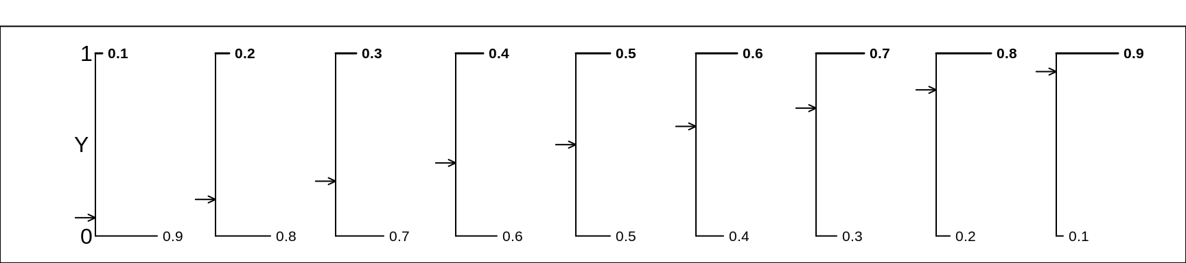
Various Bernoulli random variables/distributions. We continue our convention of using the letter Y (instead of X) as the generic name for a random variable. Moreover, in keeping with this view, all of the selected Bernoulli distributions are plotted with their 2 possible values shown on the vertical axis.

Figure 13.1: Various Bernoulli random variables/distributions. We continue our convention of using the letter Y (instead of X) as the generic name for a random variable. Moreover, in keeping with this view, all of the selected Bernoulli distributions are plotted with their 2 possible values shown on the vertical axis.

Please, when reading the Wikipedia entry, replace all instances of $X$ and $x$ by $Y$ and $y$. Note also that we will use $\pi$ where Wikipedia, and some textbooks, use $p$. As much as we can, we use Greek letters for parameters and Roman letters for their empirical (sample) counterparts. Also, to be consistent, if the random variable itslef is called $Y$, then it makes sense to use $y$ as the possible relaizations of it, rather than the illogical $k$ that Wikipedia uses.]

In the sidebar, Wikipedia shows the probability mass function (pmf, the probabilities that go with the possible $Y$ values) in two separate rows, but in the text the pmf is also shown more concisely, as (in our notation)

\[f(y) = \pi^y (1-\pi)^{1-y}, \ \ y = 0, 1.\] If we wish to align with how the R software names features of distributions, we might want to switch from $f$ to $d$. R uses $d$ because it harmonizes with the probability $d$ensity function (pdf) notation that its uses for random variables on an interval scale, even though some statistical 'purists' see that as mixing terminology: they use the term probablility mass function for discrete random variables, and probablity density function for ones on an interval scale.

\[d_{Bernoulli}(y) = \pi^y (1-\pi)^{1-y}.\]

Sadly, Bernoulli does not get its own entry in R's list of named distributions, presumably because it is a special case of a binomial distribution, one where $n$ = 1. So we have to call dbinom(x,size,prob) to get the density (probability mass) function of the binomial distribution with parameters size ($n$) and prob ($\pi$), and set $n$ to 1.

The 3 arguments to dbinom(x,size,prob) are:

x: a vector of quantiles (here just 0 or/and 1),
size: the number of 'trials' (our '$n$', so 1 for Bernoulli), and
prob: the probability of 'success' on each 'trial'. We think of it as the probability that a realization of $Y4, i.e, $y$ will equal 1, or as $\pi.$)

Thus, dbinom(x=0,size=1,prob=0.3) yields 0.7, while dbinom(x=1,size=1,prob=0.3) yields 0.3 and dbinom(x=c(0,1),size=1,prob=0.3) yields the vector 0.7, 0.3.

Incidentally, please do not adopt the convention that $x$ (or our $y$) is the number of ‘successes’ in $n$ trials. It is the number of 'positives' in a sample of $n$ independent draws from a population in which a proportion $\pi$ are positive.

Expectation (E) and Variance (V) of a Bernoulli random variable.

Shortening $Prob(Y=y)$ to $P_y$, we have

From first principles, \[E[Y] = 0 \times P_0 + 1 \times P_1 = 0 \times (1-\pi) + 1 \times \pi = \pi,\] while \[V[Y] = (0-\pi)^2 \times P_0 + (1-\pi)^2 \times P_1 = \pi^2(1-\pi) + (1-\pi)^2\pi = \underline{\pi(1-\pi)}.\]

This functional form for the ('unit') variance is not entirely surprising: it is obvious from the selected distributions whon that the most concentrated Bernoulli distributions are the ones where the proportion $(\pi)$ of Y = 1 values is either close to 1 or to zero, and that the most spread out Bernoulli distributions are the ones where $\pi$ is close to 1/2. And, and a function of $\pi$, the Variance must be symmetric about $\pi$ = 1/2.

The fact that the greatest uncertainty ('entropy', lack of order or predictability) is when $\pi$ = 1/2 is one of the factors that makes sports contests more engaging when teams or players are well matched. Later, when we come to study what influences the imprecision of sample surveys, we will see that for a given sample size, the imprecision is largest when $\pi$ is closer to 1/2.

Why focus on the variance of a Bernoulli random variable? because, later, when we use the more intesting binomial distribution, we can call on first prionciples to recall what its expectation and variance are. A Binomial random variable is the sum of $n$ independently distributed Bernoulli random variables, all with the same expectation $\pi$ and unit variance $\pi(1-\pi).$ Thus its expectation ($E$) and variance ($V$) are the sums of these 'unit' versions, i.e., $E[binom.sum] = n \times \pi$ and $V[binom.sum] = n \times \pi(1-\pi).$ Moreover, again from first principles, we can deduce that if instead of a sample sum, we are interested in a sample mean (here the mean of the 0's and 1's is the sample proportion), its expected value is \[\boxed{\boxed{E[binom.prop'n] = \frac{n \pi}{n} = \pi; \ V[.] = \frac{n \pi(1-\pi))}{n^2} = \frac{\pi(1-\pi)}{n}; \ SD[.] = \frac{\sqrt{\pi(1-\pi)}}{ \sqrt{n}} = \frac{\sigma_{0,1}}{\sqrt{n}} } } \]

Note here the generic way we write the SD of the sampling distribution of a sample proportion, in the same way that we write the SD of the sampling distribution of a sample mean, as $\sigma_u/\sqrt{n},$ where $\sigma_u$ is the 'unit' SD, the standard deviation of the values of individuals. The individual values in the case of a Bernoulli randomn variable are just 0s and 1s, and their SD is $\sqrt{\pi(1-\pi)}.$ We call this SD the SD of the 0'1 and 1's, or $\sigma_{0,1}$ for short.

Notice how, even though it might look nicer and simpler to compute, and involves just 1 square root calculation, we did not write the SD of a binomial proportion as
\[SD[binom.proportion] = \sqrt{\frac{\pi(1-\pi)}{ n} }.\] We choose instead to use the $\sigma/\sqrt{n}$ version, to show that it has the same form as the SD for the sampling distribution of a sample mean. Now that we no longer need to savw keystrokes on a hand caloculator, we should move away from computational forms and focus instead on the intuitive form. Sadly, many textbooks re-use the same concept in disjoint chapters without telling readers they are cases of the same SD formula.

There is a lot to be gained by thinking of proportions as means, but where the $Y$ values are just 0's and 1's. You can use the R code below to simulate a very large number of 0's and 1's, and calculate their variance. The sd function in R doesn't know or care that the values you supply it are limited to just 0s and 1s, or spread along an interval. Better still don't use the rbinom function; instead use the sample function, with replacement.

n = 750

zeros.and.ones = sample(0:1, n , 
   prob=c(0.2, 0.8),replace=TRUE )

m = matrix(zeros.and.ones,n/75,75)
noquote(apply(m,1,paste,collapse=""))

##  [1] 111111111110011111111111111111101111111110011101010111111011011101001000110
##  [2] 110011111111111111111111001011111011100111011101111101011101111111111111011
##  [3] 011011110111111111101111011111110111011111000111011111101110111101101011101
##  [4] 110100011111111111011111111011111111111111111101101101111110010011111111111
##  [5] 101111011111101011111111110111011110110111111110011011011010111111010111111
##  [6] 111110111111110010101111111111111101111110001111111111100110110111110110111
##  [7] 011111101111110111111111110111111110011101111111101111110111111111111110011
##  [8] 111110111101010111111111110101101110111010111100111101010110101001001010100
##  [9] 110111100111111100111001111111101111111110101010110101101111111111000111111
## [10] 011111011111111011111101111111011010001011111010101101111000100111111011111

sum(zeros.and.ones)/n

## [1] 0.7786667

round( sd(zeros.and.ones),4)

## [1] 0.4154

Try the above code with a larger $n$ and a different $\pi$ and convince yourself that the variance (and thus the SD) of the individual 0 and 1 values (a) have nothing to do with how many there are and everything to do with what proportion of them are of each type and (b) are larger when the proportions are close to each other, and smaller when they are not.

Scaled-Bernoulli random variables (to come)

Could we get by without studying the Binomial Distribution? The answer is 'for most applications, yes.' The reason is that in in most cases, we are able to use a Gaussian (Normal) approximation to the binomial distribution. Thus, all we need are its expectation and variance (standard deviation): we don't need the dbinom() probability mass function, or the pbinom() that gives the cumulative distribution function and thus the tail areas, or the qbinom() function that gives the quantiles. But sometimes we deal with situations where the binomial distributions are not symmetric and close-enough-to-Gaussian.

Below we recount how, in 1738, almost 4 decades before Gauss was born, when summing the probabilities of a binomial distribution with a large $n$, deMoivre effectively used the as-yet unrecognized 'Gaussian' distribution as a very accurate approximation. Without calling it this, he relied on the standard deviation of the binomial distribution.

===

13.2.2 Binomial

The Binomial Distribution is a model for the (sampling) variability of a proportion or count in a randomly selected sample

The Binomial Distribution: what it is

The $n+1$ probabilities $p_{0}, p_{1}, ..., p_{y}, ..., p_{n}$ of observing $y$ = $0, 1, 2, \dots , n$ 'positives' in $n$ independent realizations of a Bernoulli random variable $Y$with probability, $\pi,$ that Y=1, and (1-$\pi$) that it is 0. The number is the sum of $n$ independen Bernoulli random variables with the same probability, such as in s.r.s of $n$ individuals.
Each of the $n$ observed elements is binary (0 or 1)
There are $2^{n}$ possible sequences ... but only $n+1$ possible values, i.e. $0/n,\;1/n,\;\dots ,\;n/n$ can think of $y$ as sum of $n$ Bernoulli r. v.'s. [Later on, in ptractive, we will work in the same scale as parameter. i.e., (0,1). not the (0,n) 'count' scale.]
Apart from $n$, the probabilities $p_{0}$ to $p_{n}$ depend on only 1 parameter:
the probability that a selected individual will be 'positive' i.e., have the trait of interest
the proportion of 'positive' individuals in the sampled population
Usually we denote this (un-knowable) proportion by $\pi$ (or sometimes by the more generic $\theta$)
Textbooks are not consistent (see below); we try to use Greek letters for parameters,
Note Miettinen's use of UPPER-CASE letters, [e.g. $P$, $M$] for PARAMETERS and lower-case letters [e.g., $p$, $m$] for statistics (estimates} of parameters).

Author(s)	PARAMETER	Statistic
Clayton and Hills	$\pi$	$p = D/n$
Moore and McCabe, Baldi and Moore	$p$	$\hat{p} = y/n$
Miettinen	$P$	$p = y/n$
This book	$\pi$	$p = D/n$

Shorthand: $Y \sim Binomial(n, \pi)$ or $y \sim Binomial(n, \pi)$

How it arises

Sample Surveys
Clinical Trials
Pilot studies
Genetics
Epidemiology

Uses

to make inferences about $\pi$ from observed proportion $p = y/n$.
to make inferences in more complex situations, e.g. ...
Prevalence Difference: $\pi_{index.category}$ - $\pi_{reference.category}$
Risk Difference (RD): $\pi_{index.category}$ - $\pi_{reference.category}$
Risk Ratio, or its synonym Relative Risk (RR): $\frac{\pi_{index.category}}{\pi_{reference.category}}$
Odds Ratio (OR): $\frac{\pi_{index.category}/(1-\pi_{index.category})}{ \pi_{reference.category}/(1-\pi_{reference.category}) }$
Trend in several $\pi$'s

Requirements for $Y$ to have a Binomial$(n, \pi)$ distribution

Each element in the 'population' is 0 or 1, but we are only interested in estimating the proportion ($\pi$) of 1’s; we are not interested in individuals.
Fixed sample size $n$.
Elements selected at random and independent of each other; each element in population has the same probability of being sampled: i.e., we have $n$ independent Bernoulli random variables with the same expectation (statisticians say 'i.i.d' or 'independent and identically distributed').
It helps to distinguish the population values, say $Y_1$ to $Y_N$, from the $n$ sampled values $y_1$ to $y_n$. Denote by $y_i$ the value of the $i$-th sampled element. Prob[$y_i$ = 1] is constant (it is $\pi$) across $i$. In the What proportion of our time do we spend indoors? example, it is the random/blind sampling of the temporal and spatial patterns of 0s and 1s that makes $y_1$ to $y_n$ independent of each other. The $Y$'s, the elements in the population can be related to each other [e.g. there can be a peculiar spatial distribution of persons] but if elements are chosen at random, the chance that the value of the $i$-th element chosen is a 1 cannot depend on the value of $y_{i−1}$ or any other $y$: the sampling is 'blind' to the spatial location of the 1’s and 0s.

Binomial probabilities, illustrated using a Binomial Tree

From 5 (independent and identically distributed) Bernoulli observations to Binomial(n=5), with the Bernoulli probability left unspecified. There are 2 to the power n possible (distinct) sequences of 0's and 1's, each with its probability. We are not interested in these 2 to the power n probabilities, but in the probability that the sample contains y 1's and (n-y) 0's. There are only (n+1) possibilities for y, namely 0 to n. Fortunately, each of the n.choose.y sequences that lead to the same sum or count y, has the same probability. So we group the 2.to.power.n sequences into (n+1) sets, according to the sum or count. Each sequence in the set with y 1's and (n-y) 0's has the same probability, namely the prob.to.the.power.y times (1-prob).to.the.power.(n-y). Thus, in lieu of adding all such probabilities, we simply multiply this probability by the number, n.choose-y -- shown in black -- of unique sequences in the set. Check: the frequencies in black add to 2.to.power.n. Nowadays, the (n+1) probabilities are easily obtained by supplying a value for the 'prob' argument in the R function dbinom(), instead of computing the binomial coefficient n.choose-y by hand.

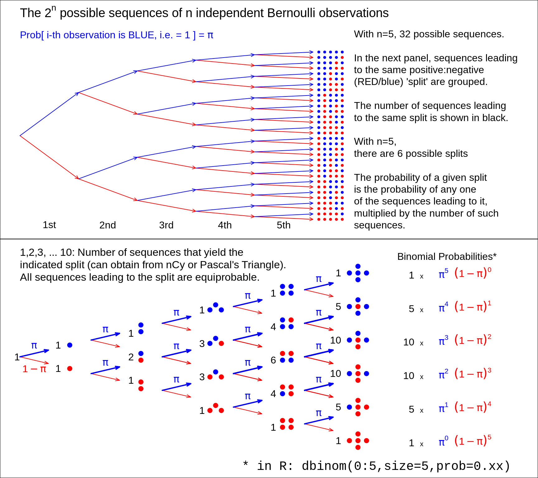
Figure 13.2: From 5 (independent and identically distributed) Bernoulli observations to Binomial(n=5), with the Bernoulli probability left unspecified. There are 2 to the power n possible (distinct) sequences of 0's and 1's, each with its probability. We are not interested in these 2 to the power n probabilities, but in the probability that the sample contains y 1's and (n-y) 0's. There are only (n+1) possibilities for y, namely 0 to n. Fortunately, each of the n.choose.y sequences that lead to the same sum or count y, has the same probability. So we group the 2.to.power.n sequences into (n+1) sets, according to the sum or count. Each sequence in the set with y 1's and (n-y) 0's has the same probability, namely the prob.to.the.power.y times (1-prob).to.the.power.(n-y). Thus, in lieu of adding all such probabilities, we simply multiply this probability by the number, n.choose-y -- shown in black -- of unique sequences in the set. Check: the frequencies in black add to 2.to.power.n. Nowadays, the (n+1) probabilities are easily obtained by supplying a value for the 'prob' argument in the R function dbinom(), instead of computing the binomial coefficient n.choose-y by hand.

If you rotate the binomial tree to the right by 90 degrees, and use your imagination, you can see how it resembles the quincunx constructed by Francis Galton. He used it to show how the Central Linit Theorem, applied to the sum of several 'Bernoulli deflections to the right and left', makes a Binomial distribution approach a Gaussian one. Several games and game shows are built on this pinball machine, for example, Plinko and, more recently, The Wall. Galton's quincunx has its own cottage industry, and versions of it often displayed in Science Museums. The present authors inherited a low tech version of the Galton Board, where the 'shot' are turnip seeds, from former McGill Professor -- and early teacher of course 607 -- FDK Liddell.

Calculating Binomial probabilities

Exactly

probability mass function (p.m.f.) :
formula: $Prob[y] = \ ^n C _y \ \pi^y \ (1 − \pi)^{n−y}$.
recursively: $Prob[0] = (1−\pi)^n$; $Prob[y] = \frac{n−y+1}{y} \times \frac{\pi}{1-\pi} \times Prob[y−1]$.
Statistical Packages:
R functions dbinom(), pbinom(), qbinom()
probability mass, distribution/cdf, and quantile functions.
Stata function Binomial(n,k,p)
SAS PROBBNML(p, n, y) function
Spreadsheet — Excel function BINOMDIST(y, n, π, cumulative)
Tables: CRC; Fisher and Yates; Biometrika Tables; Documenta Geigy

Using an approximation

Poisson Distribution ($n$ large; small $\pi$)
Normal (Gaussian) Distribution ($n$ large or midrange $\pi$, so that the expected value, $n \times \pi$, is sufficiently far 'in from' the 'edges' of the scale, i.e., sufficiently far in from 0 and from $n$, so that a Gaussian distribution doesn't flow past one of the edges. The Normal approximation is good for when you don't have access to software or Tables, e.g, on a plane, or when the internet is down, or the battery on your phone or laptop had run out, or it takes too long to boot up Windows!).
To use the Normal approximatiom, be aware of the scale you are working in, .e.g., if say $n = 10$, whether the summary is a count or a proportion or a percentage.

	r.v.	e.g.	E	S.D.
count:	$y$	2	$n \times \pi$	$\{n \times \pi \times (1-\pi) \}^{1/2}$
				i.e., $n^{1/2} \times \sigma_{Bernoulli}$

proportion:	$p=y/n$	0.2	$\pi$	$\{\pi \times (1-\pi) / n \}^{1/2}$
				i.e., $\sigma_{Bernoulli} / n^{1/2}$

percentage:	$100p\%$	20%	$100 \times \pi$	$100 \times SD[p]$

The first person to suggest an approximation, using what we now call the 'Normal' or 'Gaussian' of 'Laplace-Gaussian' distribution, was deMoivre, in 1738. There is a debate among historians as to whether this marks the first description of the Normal distribution: the piece does not explicitly point to the probability density function $\frac{1}{\sigma \sqrt{2 \pi}} \times exp[-z^2/2\sigma^2],$ but it does highlight the role of the quantity $(1/2) \times \sqrt{n}$, the standard deviation of the sum of $n$ independent Bernoulli random variables, each with expectation 1/2 and thus a 'unit' standard deviation of 1/2, and also the SD quantity $\sqrt{\pi(1-\pi)}$ $\times$ $\sqrt{n}$ in the more general case. DeMoivre arrived at the familiar '68-95-99.7 rule' : the percentages of a normal distribution that lie within 1, 2 and 3 SD's of its mean.

Factors that modulate the shapes of Binomial distributions

size of $n$: the larger the n, the more symmetric
value of $\pi$: the closer to 1/2, the more symmetric

In these small-$n$ contexts, only those distribtions where $\pi$ is close to 0.5 are reasonably symmetric.

In larger-$n$ contexts (see below), as long as there is 'room' for them to be, binomial distribtions where the expected value $E = n \times \pi$ is at least 5-10 'in from the edges' (i.e. to the right of 0, or the left of $n$, are reasonably symmetric.

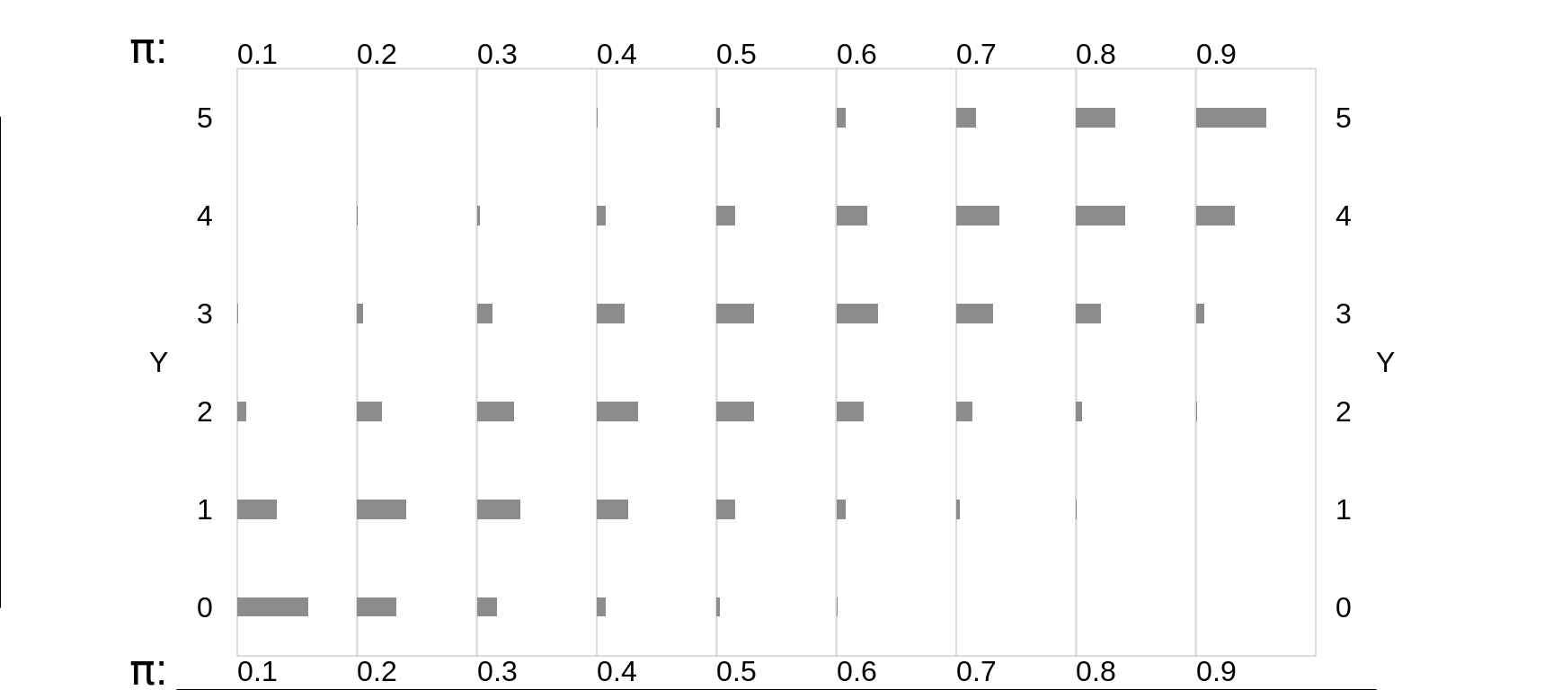
Binomial random variables/distributions, where n = 5, and the Bernoulli expectation (probability) is smaller (left panels) or larger (right panels).

Figure 13.3: Binomial random variables/distributions, where n = 5, and the Bernoulli expectation (probability) is smaller (left panels) or larger (right panels).

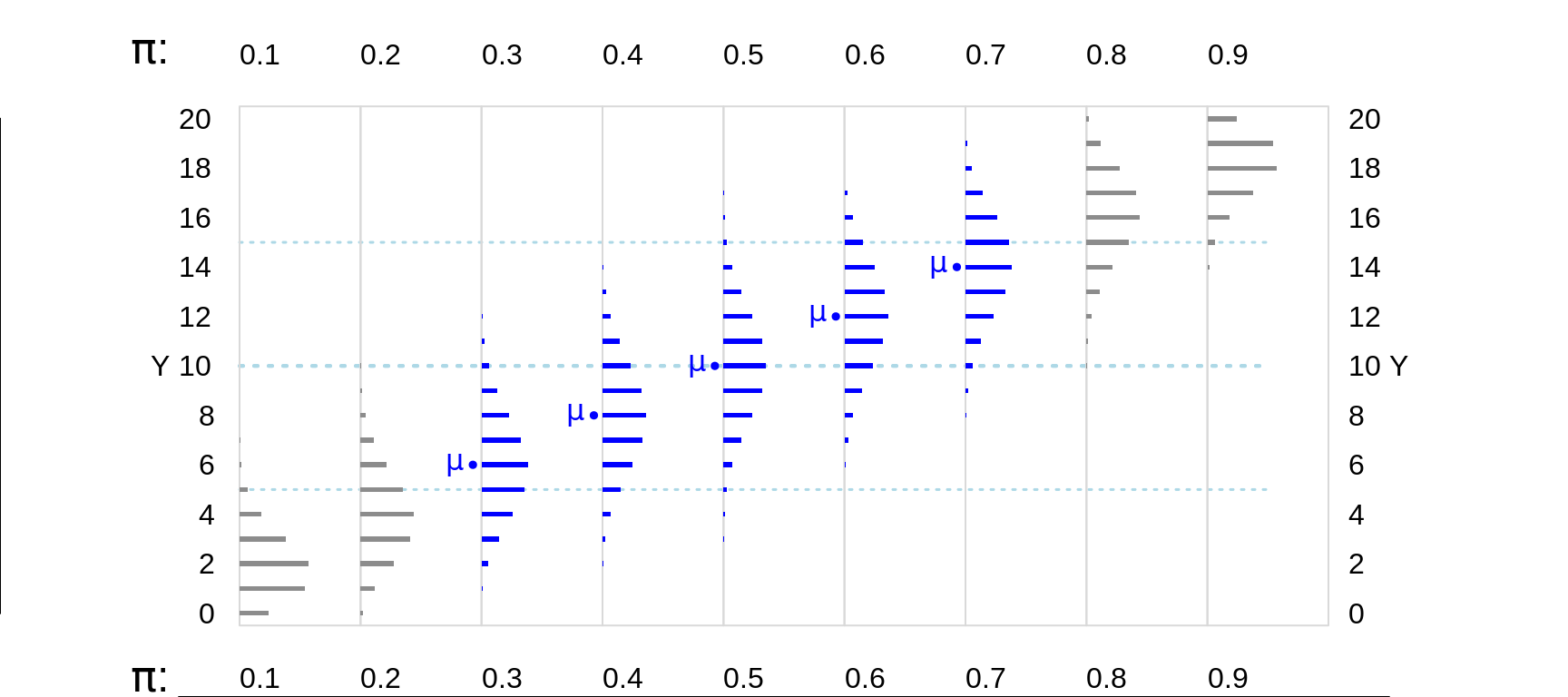
Various Binomial random variables/distributions, where n = 20. The dotted horizontal lines in light blue are 5 and 10 units in from the (0,n) boundaries. The distributions where the expected value E or mean, mu ( = n * Bernoulli Probability) is at least 5 units from the (0,n) boundaries are shown in blue.

Figure 13.4: Various Binomial random variables/distributions, where n = 20. The dotted horizontal lines in light blue are 5 and 10 units in from the (0,n) boundaries. The distributions where the expected value E or mean, mu ( = n * Bernoulli Probability) is at least 5 units from the (0,n) boundaries are shown in blue.

Various Binomial random variables/distributions, where n = 50. The blue dotted lines are 5 and 10 units in from the (0,n) boundaries. The distributions where the expected value E or mean, mu ( = n * Bernoulli Probability) is at least 5 units in from the (0,n) boundaries are shown in blue

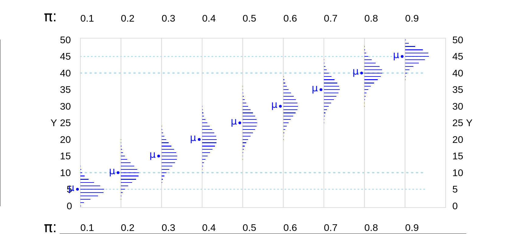
Figure 13.5: Various Binomial random variables/distributions, where n = 50. The blue dotted lines are 5 and 10 units in from the (0,n) boundaries. The distributions where the expected value E or mean, mu ( = n * Bernoulli Probability) is at least 5 units in from the (0,n) boundaries are shown in blue

Back when binomial computations were difficult, and the normal approximation was not accurate, there was another approximation that saved labour, and in particular, avoided having to deal with the very large numbers involved in the $^nC_y$ binomial coefficients (even if built into a hand calculator, these can be problematic when $n$ is large).

Poisson, in 1837, having shown how to use the Normal distribution for binomial (and the closely-related negative binomial) calculations, devoted 1 small section (81) of less than 2 pages, to the case where (in our notation) one of the two chances $\pi$ or $(1-\pi)$ 'est très petite' [Poisson's $q$ is our $\pi$, his $\mu$ is our $n$, his $\omega$ is our $\mu$, and his $n$ is our $y$]. In our notation, he arrived at \[Prob[y \ or \ fewer \ events] = \bigg(1 + \frac{\mu}{1!} + \frac{\mu^2}{2!} + \dots + \frac{\mu^y}{y!} \bigg) \ e^{-\mu}.\]

In the last of his just three paragraphs on this digression, he notes the probability $e^{-\mu}$ of no event, and $1 - e^{-\mu}$ of at least 1. He also calculates that, when $\mu$ = 1, the chance is very close to 1 in 100 million that more than $y$ = 10 events would occur in a very large series of trials (of length $n$), where the probability is 1/$n$ in each trial. Although he give little emphasis to his formula, and no real application, it is Poisson's name that is now undividely associated with this formula.

Below are some examples of how well it approximates a Binomial in the 'corner' where $\pi$ is very small and $n$ is very large. If, of course, the product, $\mu = n \times \pi$ , reaches double digits, the Normal approximation distribution provides and accurate approximation for both the Binomial and the Poisson distributions, and -- if one has ready acccess to the tail areas of a Normal distribution -- with less effort. Today, of course, unless you are limited to a hand calculator when the internet and R and paper tables are nor available, you would not need to use any approximation, Normal or Poisson, to a binomial.

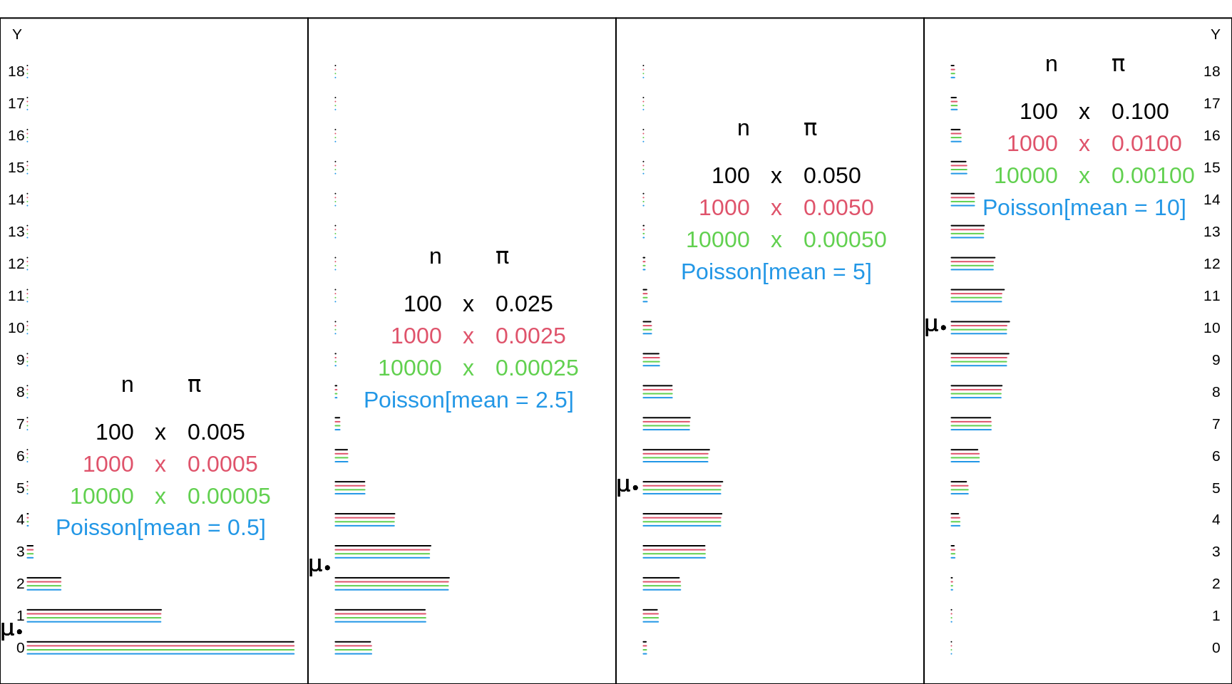
Various Binomial random variables/distributions, with large n's and small Bernoulli probabilities, together with the Poisson distributions with the corresponding means. The Poisson distrubution provides a good approximation in the 'lowee corner of the Bimonial distribution with large n's and small probabilities. And, when the product, mu = n * probability, is in the double digits, the Normal approximation distribution provides and accurate approximation for both the Binomial and the Poisson distributions.

Figure 13.6: Various Binomial random variables/distributions, with large n's and small Bernoulli probabilities, together with the Poisson distributions with the corresponding means. The Poisson distrubution provides a good approximation in the 'lowee corner of the Bimonial distribution with large n's and small probabilities. And, when the product, mu = n * probability, is in the double digits, the Normal approximation distribution provides and accurate approximation for both the Binomial and the Poisson distributions.

When the Binomial does not apply

It does not apply if one (or both) of the 'i.i.d.' (independent and identical) conditions do not hold. The first of these conditions is often the one that is absent.

Two very nice examples can be found in Cochran's (old but still excellent) textbook on sampling. They were re-visited a few decades years ago in connection with what was (then) a new technique for dealing with correlated responses.

The table shows, for each of the 30 randomly sampled households, the number of household members had visited a physician in the previous year. Can we base the precision of the observed proportion, 30/104 or 28%, on a binomial distribution where $n$ = 104?

True, the 'n' in each household is not the same from household to household, but we can segregate the households by size, and carry out separate binomial calculations for each, all the time assuming a common binomial proportion across houdeholds.

XLAB = "y: number in household who has visited an MD in last year"
YLAB = "Number of Households\nfor which y persons visited an MD"

show.household.survey.data(n.who.visited.md,XLAB,YLAB)

## [1] No. persons with history/trait of interest: 30 / 104 ; Prop'n: 0.29
## [1]  
## Below, the row labels are the household sizes.
## Each column label is the number in a household with history/trait of interest.
## The entries are how many households had the indicated configuration.
## 
##           0    1    2    3    4    5    6    7    Total
## 1         1    .    .    .    .    .    .    .        1
## 2         3    .    1    .    .    .    .    .        4
## 3         7    2    1    2    .    .    .    .       12
## 4         4    1    3    .    1    .    .    .        9
## 5         .    .    1    .    .    1    .    .        2
## 6         1    .    .    .    .    .    .    .        1
## 7         1    .    .    .    .    .    .    .        1
## Total    17    3    6    2    1    1    0    0       30
## 
## Same row/col meanings, but theoretical, binomial-based,
## EXPECTED frequencies of households having these many persons
##  who would have -- if all 128 persons were independently sampled
## from a population where the proportion with 
## the history/trait of interest was as above.
## 
##           0     1     2     3     4     5     6     7 Total
## 1     0.712 0.288     .     .     .     .     .     .     1
## 2     1.013 0.821 0.166     .     .     .     .     .     4
## 3     1.081 1.314 0.533 0.072     .     .     .     .    12
## 4     1.025 1.663 1.011 0.273 0.028     .     .     .     9
## 5     0.912 1.849 1.499 0.608 0.123 0.010     .     .     2
## 6     0.779 1.894 1.920 1.038 0.315 0.051 0.003     .     1
## 7     0.646 1.834 2.231 1.507 0.611 0.149 0.020 0.001     1
## Total 6.167 9.663 7.360 3.498 1.077 0.210 0.024 0.001    30
## 
## We will just assess the fit on the 'totals'row:
##  the numbers in the individual rows are too small to judge.
## 
##         0   1   2   3   4   5 6 7 Total
## [1,] 17.0 3.0 6.0 2.0 1.0 1.0 0 0    30
## [2,]  6.2 9.7 7.4 3.5 1.1 0.2 0 0    30
## 
## Better still, here is a picture: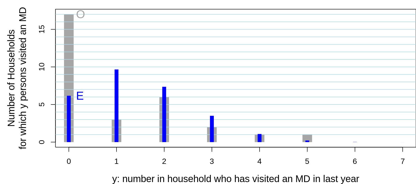

Of 30 randomly sampled households, (O)bserved numbers of households, shown in grey, where 0, 1, .. in household had visited a physician in the previous year. The 30 households contained 104 persons, 28 of whom had visited a physician in the previous year. Also shown, in blue are the (E)xpected numbers of households, assuming the data were generated from 104 independent Bernoulli random variables, each with the same probability 28/104. The observed variance is considerably LARGER than that predicted by a binomial distribution. You would see this even if the individuals in the house were not from the same family. For example, if the occupants were students, the proportion of them with such a history would be different (?lower) than if the occupants were older: this is the 'non-identical probabilities' aspect. The other possibility, the 'non-independence' aspect, is that health status and the seeking medical care are affected by shared family factors, such as behaviours, attitudes, lifestyle, and insurance coverage.

Figure 13.7: Of 30 randomly sampled households, (O)bserved numbers of households, shown in grey, where 0, 1, .. in household had visited a physician in the previous year. The 30 households contained 104 persons, 28 of whom had visited a physician in the previous year. Also shown, in blue are the (E)xpected numbers of households, assuming the data were generated from 104 independent Bernoulli random variables, each with the same probability 28/104. The observed variance is considerably LARGER than that predicted by a binomial distribution. You would see this even if the individuals in the house were not from the same family. For example, if the occupants were students, the proportion of them with such a history would be different (?lower) than if the occupants were older: this is the 'non-identical probabilities' aspect. The other possibility, the 'non-independence' aspect, is that health status and the seeking medical care are affected by shared family factors, such as behaviours, attitudes, lifestyle, and insurance coverage.

Cochran provides this explanation for the greater than binomial variation in the proportions

The variance given by the ratio method, 0.00520, is much larger than that given by the binomial formula, 0.00197. For various reasons, families differ in the frequency with which their members consult a doctor. For the sample as a whole, the proportion who consult a doctor is only a little more than one in four, but there are several families in which every member has seen a doctor. Similar results would be obtained for any characteristic in which the members of the same family tend to act in the same way.

Clearly, if we are dealing with an infectious disease, we would need to be very careful about our statistical model for the numbers in a family or household or care facility that are affected.

XLAB = "y: number of males in household"
YLAB=  "Number of Households\n where y persons were male"
show.household.survey.data(n.males,XLAB,YLAB)

## [1] No. persons with history/trait of interest: 53 / 104 ; Prop'n: 0.51
## [1]  
## Below, the row labels are the household sizes.
## Each column label is the number in a household with history/trait of interest.
## The entries are how many households had the indicated configuration.
## 
##          0     1    2    3    4    5    6    7    Total
## 1        1     .    .    .    .    .    .    .        1
## 2        .     4    .    .    .    .    .    .        4
## 3        .     7    5    .    .    .    .    .       12
## 4        .     1    3    5    .    .    .    .        9
## 5        .     1    .    1    .    .    .    .        2
## 6        .     .    .    1    .    .    .    .        1
## 7        .     .    .    1    .    .    .    .        1
## Total    1    13    8    8    0    0    0    0       30
## 
## Same row/col meanings, but theoretical, binomial-based,
## EXPECTED frequencies of households having these many persons
##  who would have -- if all 128 persons were independently sampled
## from a population where the proportion with 
## the history/trait of interest was as above.
## 
##           0     1     2     3     4     5     6     7 Total
## 1     0.490 0.510     .     .     .     .     .     .     1
## 2     0.481 1.000 0.519     .     .     .     .     .     4
## 3     0.354 1.103 1.146 0.397     .     .     .     .    12
## 4     0.231 0.962 1.499 1.038 0.270     .     .     .     9
## 5     0.142 0.737 1.531 1.591 0.827 0.172     .     .     2
## 6     0.083 0.520 1.352 1.873 1.460 0.607 0.105     .     1
## 7     0.048 0.347 1.083 1.875 1.949 1.215 0.421 0.062     1
## Total 1.829 5.178 7.130 6.775 4.505 1.994 0.526 0.062    30
## 
## We will just assess the fit on the 'totals'row:
##  the numbers in the individual rows are too small to judge.
## 
##        0    1   2   3   4 5   6   7 Total
## [1,] 1.0 13.0 8.0 8.0 0.0 0 0.0 0.0    30
## [2,] 1.8  5.2 7.1 6.8 4.5 2 0.5 0.1    30
## 
## Better still, here is a picture: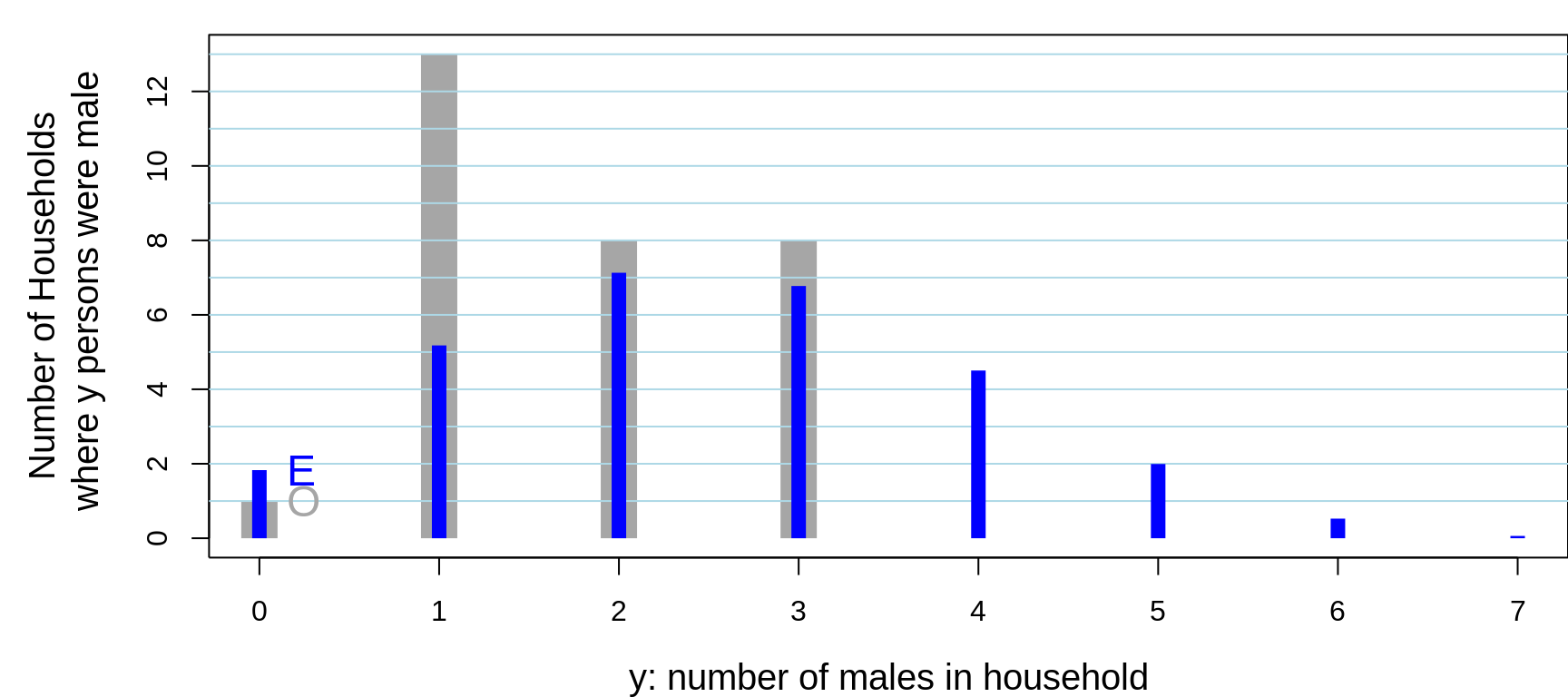

Of 30 randomly sampled households, (O)bserved numbers of households, shown in grey, where 0, 1, .. in household were male. The 30 households contained 104 persons, 53 of whom were male. Also shown, in blue are the (E)xpected numbers of households, assuming the data were generated from 104 independent Bernoulli random variables, each with the same probability 53/104. The observed variance is considerably SMALLER than that predicted by a binomial distribution. You would see this even if the individuals in the house were not from the same family. For example, if the occupants were students, the proportion of them with such a history would be different (?lower) than if the occupants were older: this is the 'non-identical probabilities' aspect. The other possibility, the 'non-independence' aspect, is that health status and the seeking medical care are affected by shared family factors, such as behaviours, attitudes, lifestyle, and insurance coverage.

Figure 13.8: Of 30 randomly sampled households, (O)bserved numbers of households, shown in grey, where 0, 1, .. in household were male. The 30 households contained 104 persons, 53 of whom were male. Also shown, in blue are the (E)xpected numbers of households, assuming the data were generated from 104 independent Bernoulli random variables, each with the same probability 53/104. The observed variance is considerably SMALLER than that predicted by a binomial distribution. You would see this even if the individuals in the house were not from the same family. For example, if the occupants were students, the proportion of them with such a history would be different (?lower) than if the occupants were older: this is the 'non-identical probabilities' aspect. The other possibility, the 'non-independence' aspect, is that health status and the seeking medical care are affected by shared family factors, such as behaviours, attitudes, lifestyle, and insurance coverage.

Cochran provides this explanation for the (unsually) less than binomial variation seen in this response variable.

In estimating the proportion of males in the population, the results are different. By the same type of calculation, we find binomial formula: v(p) = 0.00240; ratio formula v(p) = 0.00114
Here the binomial formula overestimates the variance. The reason is interesting. Most households are set up as a result of a marriage, hence contain at least one male and one female. Consequently the proportion of males per family varies less from one half than would be expected from the binomial formula. None of the 30 families, except one with only one member, is composed entirely of males, or entirely of females. If the binomial distribution were applicable, with a true P of approximately one half, households with all members of the same sex would constitute one quarter of the households of size 3 and one eighth of the households of size 4. This property of the sex ratio has been discussed by Hansen and Hurwitz (1942). Other illustrations of the error committed by improper use of the binomial formula in sociological investigations have been given by Kish (1957).

Does the Binomial Distribution apply if... ?

Interested in:	$\pi$	the proportion of 16 year old girls in Quebec protected against rubella
Choose:	$n$ = 100	girls: 20 at random from each of 5 randomly selected schools ['cluster' sample]
Count	$y$	how many of the $n$ = 100 are protected
		$\bullet$ Is $y ~ \sim Binomial(n=100, \ \pi)$ ?
.............	...........	...............................................................
'SMAC':	$\pi$	Chemistry Auto-analyzer with n = 18 channels. Critertion for 'positivity' set so that Prob['abnormal' result in Healthy person] = 0.03 for each of 18 chemistries tested

Count	$y$	(In 1 patient) how many of $n$ = 18 give abnormal result.

		$\bullet$ Is $y ~ \sim Binomial(n=18, \ \pi=0.03)$ ? credit: Ingelfinger textbook
.............	...........	...............................................................
.............	...........	...............................................................
Sex Ratio:	$n=4$	children in each family
	$y$	number of girls in family
		$\bullet$ Is $y ~ \sim Binomial(n=4, \ \pi=0.49)$ ?
.............	...........	...............................................................
Interested in:	$\pi_u$	proportion in 'usual' exercise classes and in
	$\pi_e$	expt'l. exercise classes who 'stay the course'
Randomly	4	classes of
Allocate	25	students each to usual course
	$n_u = 4 \times 25 = 100$

	$n_e$ = 4	classes of
	25	students each to experimental course
	$n_e = 4 \times 25 =100$

Count	$y_u$	how many of the $n_u$ = 100 complete course
	$y_e$	how many of the $n_e$ = 100 complete course
		$\bullet$ Is $y_u ~ \sim Binomial(n = 100, \ \pi_u)$ ?
		$\bullet$ Is $y_e ~ \sim Binomial(n = 100, \ \pi_e)$ ?
.............	...........	...............................................................
Pilot Study:		To estimate proportion $\pi$ of population that is eligible and willing to participate in long-term research study, keep recruiting until obtain
	$y$ = 5	who are. Have to approach $n$ to get $y$.
		$\bullet$ Is $y ~ \sim Binomial(n, \ \pi)$ ?
.............	...........	...............................................................

13.2.3 Poisson

model for (Sampling) Variability of a Count in a given amount of 'experience'

Today, Poisson's distribution is seldom used as a computational shortcut to a binomial probability. Although Poisson did not appreciate it at the time, today his distribution has to do with the distribution of counts of events in a given amount of space or time or population-time. However, most mathematical statistics textbooks still derive the Poisson distribution as the limiting case of a Binomial.

Below, we will take a broader view, emphasize the 'time' dimension, and give some history. We will also focus on the many contexts when the Poisson distribution is too narrow, and thus an inappropriate model for counts. We will repeat the earlier message that just because a random variable involves counts doesn't make its distribution Poisson. Examples of this include the fallacy of treating the distributions of white blood cell, or CD4 cell concentrations as if there were observed counts. And even if they are 'real' counts, the distribution (variability) of one's step-counts acrross the day or across days, or of the numbers of births or deaths or car-crashes across the day, or across days, are usually far-from-Poisson.

Indeed, we will take the attitude that counts rarely follow a Poisson distribution.

The Poisson Distribution: what it is, and some of its features

The (infinite number of) probabilities $P_{0}, P_{1}, ..., P_{y}, ...,$ of observing $Y = 0, 1, 2, \dots , y, \dots$ 'events'/'instances' in a given amount of 'experience.'
These probabilities, $Prob[Y = y]$, or $P_{Y}[y]$'s, or $P_{y}$'s for short, are governed by a single parameter, the mean $E[Y] = \mu.$
$P[y]= \exp[-\mu]\: \frac{\mu^{y}}{y!};$ in R: dpois( ) -- too bad $\mu$ is referred to as lambda.
Shorthand: $Y\sim\; \textrm{Poisson}(\mu)$.
$\sigma^2_Y = \textrm{Variance}[Y] = \mu \ ; \ \ \sigma_Y = \sqrt{\mu_{Y}}.$
It can be approximated by $N(\mu, \: \sigma_{Y} = \mu^{1/2})$ when $\mu >> 10$.
It is open-ended (unlike Binomial), but in practice, has finite range.
Poisson data are sometimes called 'numerator only': (unlike in the Binomial) you may not 'see' or count 'non-events': but there is (an invisible) denominator 'behind' the number of 'wrong number' phone calls you receive.

How it arises / derivations

Count of events (items) that occur randomly, with low homogeneous intensity, in time, space, or 'item'-time (e.g. person--time).
As a limiting case of a Binomial($n,\pi$) when $n \rightarrow \infty\textrm{ and } \pi \rightarrow 0,$ but $n \times \pi = \mu$ is finite. [Poisson, in 1837, derived it as an approximation to the closely-related negative binomial distribution.]
$Y\sim Poisson(\mu_{Y}) \Leftrightarrow T \textrm{ time between events}\sim \: \textrm{Exponential}(\mu_{T} = 1/\mu_{Y}).$ Here is one attempt to explain this and here is another together with this translation and additional annotation
As the sum of $\ge 2$ independent Poisson rv's, with the same or different $\mu$'s:
$Y_{1} \sim \textrm{Poisson}(\mu_{1}) \: \: Y_{2} \sim \textrm{Poisson}(\mu_{2}) \Rightarrow Y = Y_{1} + Y_{2} \sim \textrm{Poisson}(\mu_{1}+\mu_{2}).$
Examples: numbers of asbestos fibres, deaths from horse kicks, needle-stick or other percutaneous injuries, bus-driver accidents, twin-pairs, radioactive disintegrations, flying-bomb hits*, white blood cells, typographical errors, 'wrong numbers', cancers; chocolate chips, radioactive emissions in nuclear medicine, cell occupants -- in a given volume, area, line-length, population-time, time, etc. * included in

Calculating Poisson probabilities:

Exactly
R: dpois, ppois, qpois rpois mass/cum./quant./rand
`SAS: POISSON;
`Stata:
Spreadsheet --- Excel function POISSON} ($y, \mu$, cumulative)
Using Gaussian Approximations to distribution of $y$ or transforms of it: described below, under Inference.
In 'the old days' i.e. in the years BC (Before Computers'), Poisson tail probabilities were often calculated using links to the tail areas of other better-tabulated continuous distributions, such as the Chi-Square distribution.

Some History (see Haight ).

1718 deMoivre : the series $e^{-\mu} \bigg(1 + \frac{\mu}{1!} + \frac{\mu^2}{2!} + \dots \bigg)$ appears.
1837 Poisson (see above)
1860 Simon Newcomb, a Canadian-born 'astronomer, applied mathematician and autodidactic polymath who who was Professor of Mathematics in the United States Navy and at Johns Hopkins University, derives the 'Poisson' Law 'from scratch' as a limiting case of the Binomial, and applies it to the determination of the 'probability that, if the stars were scattered at random over the heavens, any small space selected at random would contain $s$ stars.'
1878 Abbe determined the number of cells one needed to count in order to achieve a sufficiently small 'probable error' for an estimated blood cell concentration.
1905 Schweidler provided error calculations for counting radioactive transformations.
1989 Bortkewitsch book, with many examples, and tables of the Poisson Distribution.
1907 'Student' derived the Poisson distribution from scratch (as a liniting case of the binomial) and provided error calculations for measuring yeast cells in beer.
1909 Erlang, a Danish engineer concerned with the theory of telephone traffic, developed the Poisson Law by an elegant argument based on the steady state behaviour of the beginning and terminations of calls. Here are the original Danish version and a translation. This 'simple explanation' in the English translation of a 1920 article has a critical cut and paste typographical error. The original Danish version has it correct.
1910 Rutherford (having departed McGill in 1907) and Geiger (of the 'counter'), physicists, and Bateman, a mathematician, developed the Poisson Law by an time-based argument expressed as a differential equation, a Law that agreed with the empirical distibution in their large particle-counting experiment.
1946 Flying-bomb attacks on London during WW II, along with 2019 Update: Significance Magazine Early-career Writing Award announcement and intro to and full article.
Commentators:
Newbold gives a lot of credit to deMoivre.
Haight is the mots comprehensive.
Stigler is a bit more nuanced.

13.2.3.1 DETAILED EXAMPLE 1: Distribution of particles in volumes

The following two distributions are taken from 'Student's 1907 article on counting yeast cells under a haemocytometer, an instrument for visual counting of the number of cells in a blood sample or other fluid under a microscope. In the article, he derived what today we would call the Poisson distribution, and offered guidance on how many fields/cells to count in order the ensure a small enough margin of error when estimating a concentration.

Student's main messages

The same accuracy is obtained by counting the same number of particles whatever the dilution. Hence the most accurate way is to dilute the solution to the point at which the particles may be counted most rapidly, and to count as many as time permits.

The standard deviation of the mean number of particles per unit volume is $\sqrt{m/M},$ where $m$ is the mean number and M the number of unit volumes counted.

This theoretical work was tested on four distributions which had been counted over the whole 400 squares of the haemocytometer. The particles counted were yeast cells which were killed by adding a little mercuric chloride to the water in which they had been shaken up. A small quantity of this was mixed with a 10% solution of gelatine, and after being well stirred up drops were put on the haemacytometer. This was then put on a plate of glass kept at a temperature just above the setting point of gelatine and allowed to cool slowly till the gelatine had set. Four different concentrations were used. The full description can be found here.

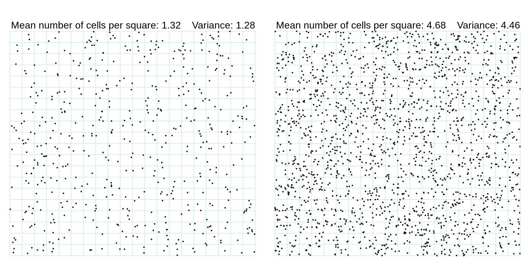
Examples of distributions of Yeast Cells over 1 sq. mm. divided into 400 squares. The data in the right panel are based on the 400 counts in Table 1 of Student's article (concentration IV), while those in the left panel are simulated to match the reported mean (1.32 per square) and variance (1.28) for the 400 counts at concentration II. It appears that Student calculated the variance using a divisor of n rather than n-1.

Figure 13.9: Examples of distributions of Yeast Cells over 1 sq. mm. divided into 400 squares. The data in the right panel are based on the 400 counts in Table 1 of Student's article (concentration IV), while those in the left panel are simulated to match the reported mean (1.32 per square) and variance (1.28) for the 400 counts at concentration II. It appears that Student calculated the variance using a divisor of n rather than n-1.

The data in the panel on the right panel can be viewed at the bottom of this page.

If we were asked to randomly distribute items over the 400 squares and have the means and standard distribitions match the observed ones, but to do it without the aid of a formal statistical procedure, most of us would do a poor job. Humans are not very good at making up random sequences. (see elsewhere, in the computing exercises). JH tested this a few decades ago by asking elementary school students to mark six spots on a 6-49 ticket -- when it uses to be mainly played using paper tickets, the 49 numbers were laid our as a 5 x 10 grid. They, and adults likewise, tend to avoid the 'border cells' and choose more in the middle of the grid.

Likewise, people are not good at detecting non-randomness. (Without peeking at the statistical summaries under row A, or at row B or at row C, or elsewhere in the article) see if you can spot the non-randomness in one of the 3 panels (1969, 1970 1971) in row (A) of Figure 4 in this article.. Hint: one of the 3 has a problem. and see if you would make a good radiologist.

Student shook the liquid vigorously and took care to avoid 'clumping' of cells, and other artifacts, and measured the (as they turned out to be, small) correlations between the nunber of cells on a square and the number in each of the four cells nearest it.

He noticed that in both concentrations I and III the variance was greater than the mean, due to an [to us, slight] excess (of the "observed") over the calculated ("fitted") among the high numbers in the tail of the distribution. [Mean = 0.6825, variance 0.8117 in I; Mean = 1.80; variance = 1.96 in III]. He has pointed out earlier in the article that the budding of the yeast cell increases these high numbers, and there is also probably a tendency to stick together in groups which was not altogether abolished even by vigorous shaking.

He also tested the observed frequency distribution of the 400 counts (they varied from 0 to 6 in the left panel, and 1 to 12 in the right panel) against the expected numbers of 0's, 1's, 2's, etc. under the (Poisson) law using a $\chi^2$ goodness of fit statistic, and found them to be reasonable. 'The p-values, 0.04, 0.68, 0.25 and 0.64, though not particularly high, are not at all unlikely in four trials, supposing our theoretical law to hold, and we are not likely to be very far wrong in assuming it to do so.'

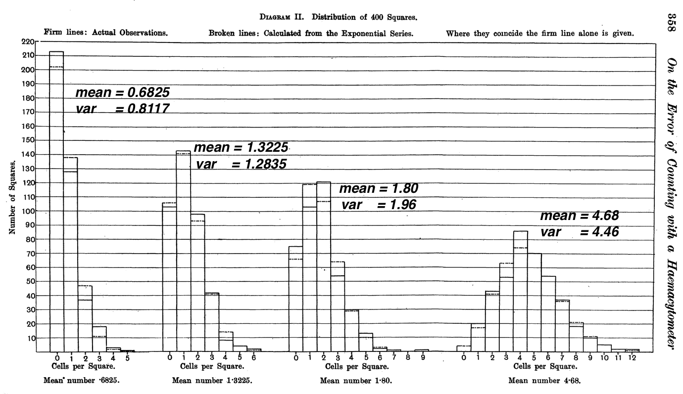
Figure 13.10: Fits of Poisson Frequencies to the 4 sets of yeast cell counts made by Student.

Clearly, the narrow pure-Poisson variation we see in Student's counts is a tribute to his 'vigorous shaking' that produced the randomness. [Think about how you would ensure this with raisins in dough, or chocolate chips in cookies.]

13.2.3.2 DETAILED EXAMPLE 2: Distribution of events in time intervals

This next example -- on counting alpha-radiation disintegrations -- has the same element of randomness, but in the time dimension. Here is Rutherford's description:

The source of radiation was a small disk coated with polonium, which was placed inside an exhausted tube, closed at one end by a zinc sulphide screen. The scintillations were counted in the usual way by means of a microscope on an area of about one sq. mm. of screen. During the timo of counting (5 days), in order to correct for the decay, the polonium was moved daily closer to the screen in order that the average number of $\alpha$ particles impinging on the screen should be nearly constant. The scintillations were recorded on a chronograph tape by closing an electric circuit by hand at the instant of each scintillation. Time-marks at intervals of one half-minute were also automatically recorded on iho same tape.
After the eye was rested, scintillations were counted from 3 to 5 minutes. The motor running the tape was then stopped and the eye rested for several minutes ; then another interval of counting, and so on. It was found possible to count 2000 scintillations a day, and in all 10,000 were recorded. The records on the tape were then systematically examined. The length of tape corresponding to half-minute marks was subdivided into four equal parts by means of a celluloid film marked with five parallel lines at equal distances. By slanting the film at different angles, the outside lines were made to pass through the time-marks, and thee number of scintillations between the lines corresponding to 1/8 minute intervals were counted through the film. By this method correction was made for slow variations in the speed of the motor during the long interval required by the observations.

The black dots on the winding line are meant to look like the marks on a 5-minute strip of the paper tape described by Rutherford.

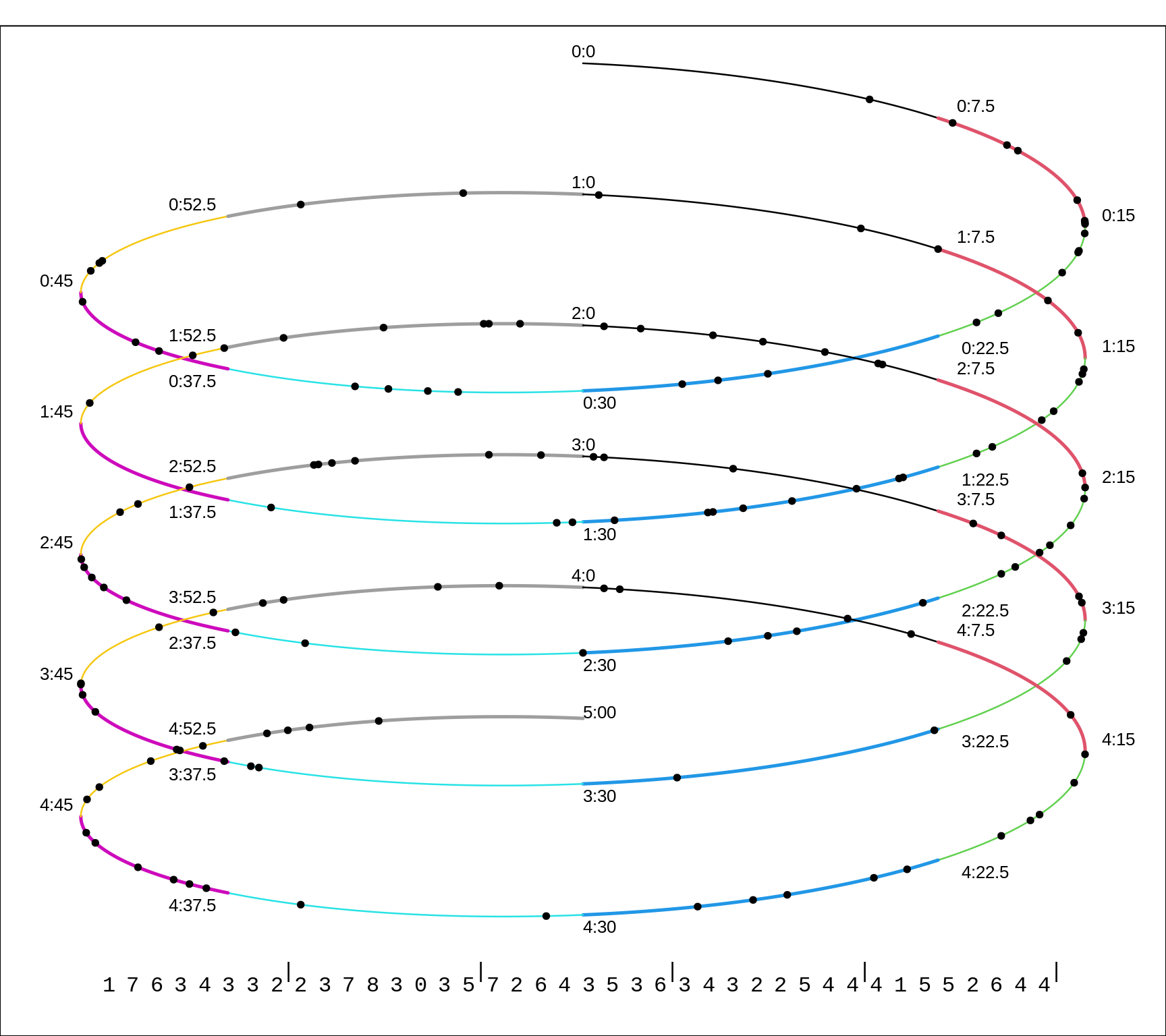
Simulated distributions of events (scintillations produced by a radioactive source) over a 5-minute time-span. Each 1/8th of a minute is shown is a different colour. The counts in each 7.5 second bin are shown at the bottom.

Figure 13.11: Simulated distributions of events (scintillations produced by a radioactive source) over a 5-minute time-span. Each 1/8th of a minute is shown is a different colour. The counts in each 7.5 second bin are shown at the bottom.

The full distribution (over 2608 intervals of 7.5 seconds duration each, i.e almost 5.5 hours in all), along with the fitted one, is graphed at the bottom of this page, and tabulated on this page.. For convenience, the two are combined in the following graph.

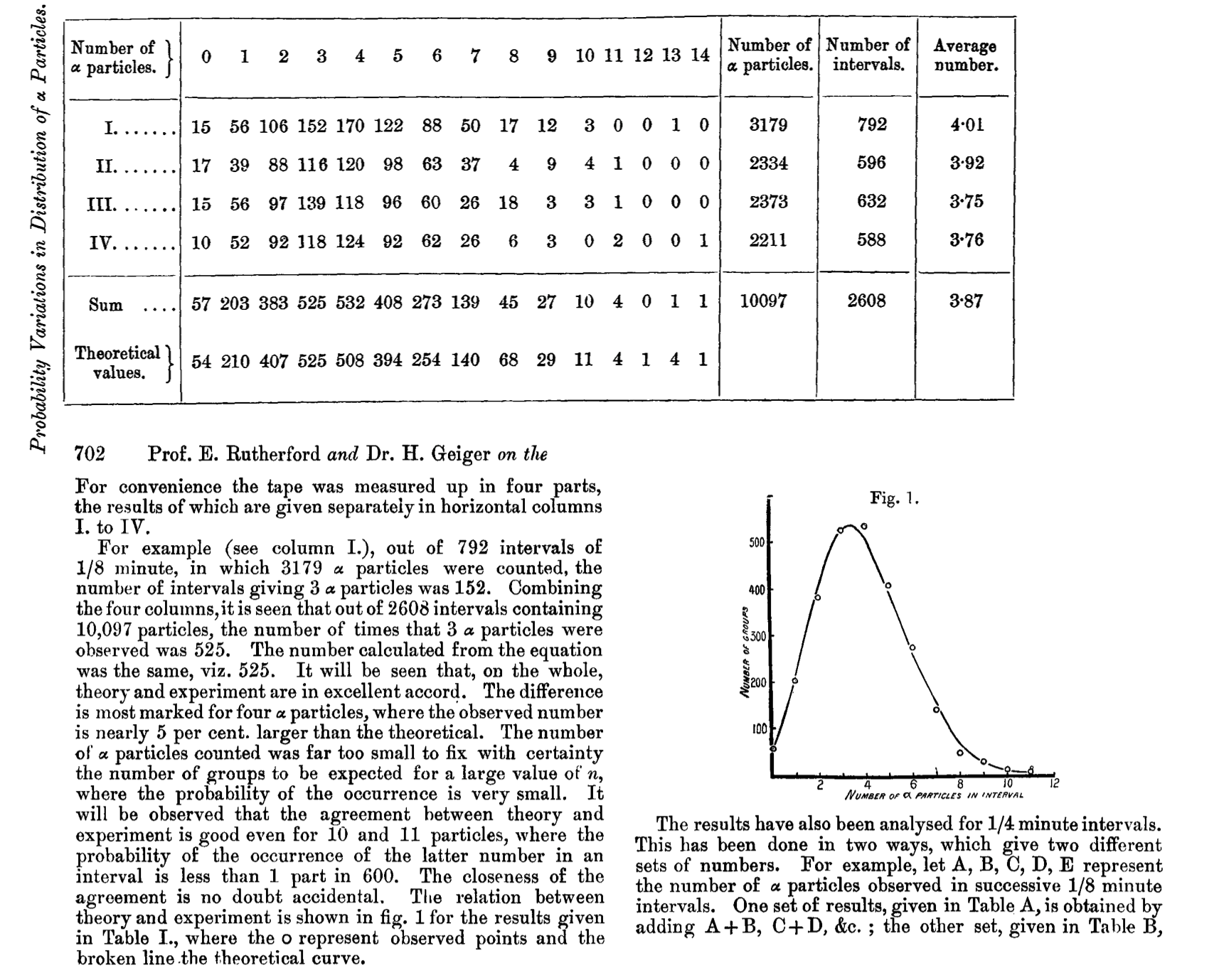
Figure 13.12: Table and Figure from Rutherford, Geiger and Bateman, 1910.

Today, we could rework his data, and replot his Figure using R.

y = 0:14; freq =c(57,203,383,525,532,408,273,139,45,27,10,4,0,1,1)

par(mfrow=c(1,1),mar = c(6,4,0,0))

plot(y,freq,
  ylab="Number of intervals",
  xlab="y: number counted in 7.5 sec interval",type="h",
  lend="butt", lwd=16,col="grey75", cex.lab=1.35)

n = sum(freq)
mean = sum(freq*y)/n
var =  sum(freq*y^2)/n - mean^2
theoretical.freq = sum(freq)*dpois(y,mean)

lines(y,theoretical.freq, type="h",
      lend="butt", lwd=6,col="blue")

text(12,400, paste("Mean(y): ",toString(round(mean,2)),
           "\nVar(y): ",toString(round(var,2)),sep=""), 
     adj=c(1,1), cex=1.5,family="mono"  )

text(5,theoretical.freq[6],"E",
     col="blue", adj=c(-1,0.5),cex=1.25)
text(5,freq[6],"O",
     col="grey65", adj=c(1.6,0.5),cex=1.25)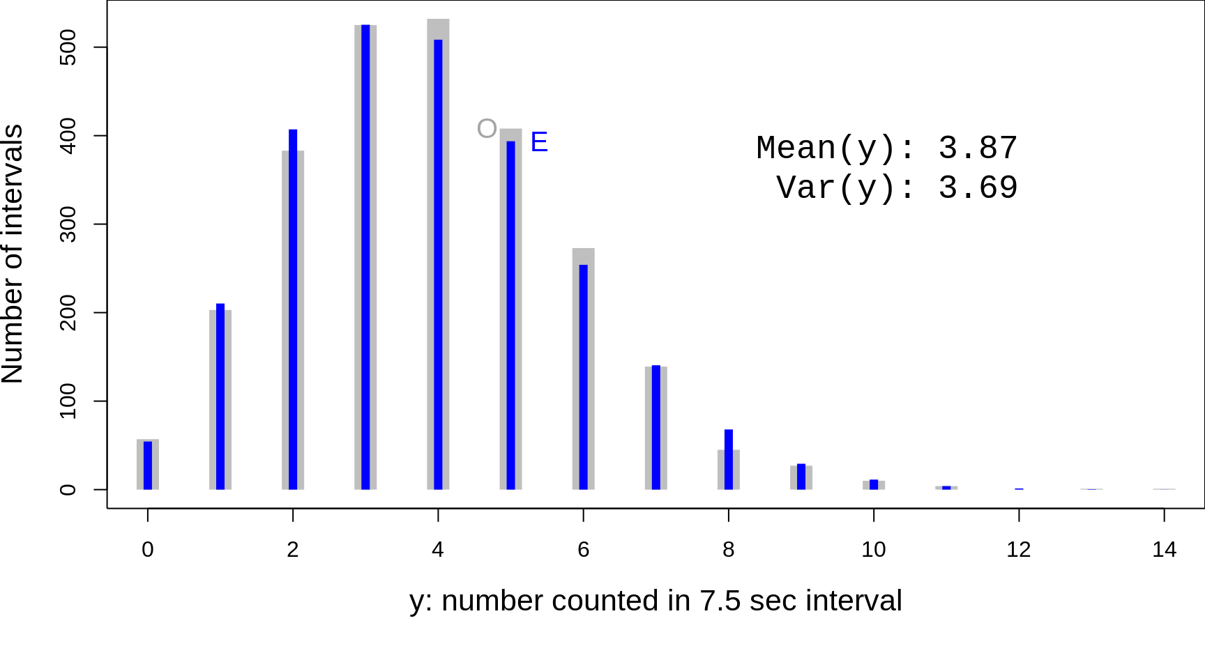

Rutherford's Fig 1, replotted, and the discrete scale emphasized. O =' 'Observed' frequencies; E = 'Expected' or 'Theoretical' or 'Fitted' frequencies. Rutherford et al. derived the theoretical distribution (blue) 'from scratch' by a very different method than Poisson (see 'Note' on pages 704-707 of their article), and made no reference to Poisson's formula.

Figure 13.13: Rutherford's Fig 1, replotted, and the discrete scale emphasized. O =' 'Observed' frequencies; E = 'Expected' or 'Theoretical' or 'Fitted' frequencies. Rutherford et al. derived the theoretical distribution (blue) 'from scratch' by a very different method than Poisson (see 'Note' on pages 704-707 of their article), and made no reference to Poisson's formula.

2020 re-enactment

This video is JH's 'recreation' of Rutherford and Geiger's experiment. Since you are unlikely to be as motivated as their 'counters', the video is limited to a 7 second lead-in + 60 seconds of flashes. If you find it easier to count while listening rather than watching, here is an audio version.

Rutherford et al. counted an average of 3.89 flashed per 7.5 seconds, or approx 0.5 per second. The video has 24 frames per second, so their average would be approx 1 per 48 frames. Thus in one frame, the expected number of flashes would be 1/48, and so one can approximate the process by modelling the result in each frame as the realization of a Bernoulli random variable, with prob = 1/48 (or slightly hogher if we wanted to more closely match their average of just over 31 flashes per minute). In theory, there could be 2 (or even 3) flashes in a 1/24 second interval, but (as we will see below when we examine the Poisson probabilities) the chances of these are small. (We could of course have make the video smoother, by having say 50 frames a second, and an average of 1 flash per 100 frames. This would diminish the chance of 2 or more flashes in a frame, but it would make the video file larger, and the higher frame rate would diminish the chance of seeing a flash in a single frame -- we haven't tested the limits of detection. We could also, of course, have put the -- very occasional -- 2 flashes in two locations in the same 1/24 sec frame.)

13.2.3.3 FROM BIOLOGICAL/PHYSICS LABORATORIES to HUMAN POPULATION-TIME

We should not automatically assume that because they also involve counts, the numbers of human events in various segments of population time wiull follow a nice tight single Poisson distribution. Student (Gosset) could distribute the yeast cells randomly by shaking them; and Rutherford could maintian the intensity of the stream of recorded atomic disintegrations constant by managing the distance between the source and the target. Such (experimental) controls are not possible in human situations that are affeceted by changing behavioural and environmental conditions.

The first example from Bortkewitsch involve termporal variations in the counts of a quite rare condition -- suicide, but there are several reasons not to equate these variations with those of Rutherford. First, they occurred over 25 years, rather than just within a total of just 5 hours spread over just five days. In that time, several things could have changed: the size of the source population might have changed somewhat; the economic and religious conditions are likely to have changed. there is the possibility of 'copycat' suicides, or multiple suicides. the attitudes to the reporting of suicide might have changed, and there must have been many more recorders/counters that the few that Rutherford used. Below, we will look at contemporary data from the USA, where many similar issues could be raised.

Note an extra feature: these events emerged from (occurred on) 2 segments of the population time .. the female population-time and the male population-time. This would be like having two radiation-counting studies proceeding simulataneously, one using polonium, and another using radium. The expected rates (the expected numbers of events per unit time) would be different.

Example 1, From Bortkewitsch, 1898

The table below contains the numbers of boys (Knaben) and girls (Mädchen) under 10 years of age in Prussia in the period 1869-1893 who committed suicide.

Jayr = 1869:1893

n.boys =c(2, 3, 1, 4, 1, 4, 0, 3, 0, 1, 2, 6, 3, 4, 1, 0, 2, 2, 1, 1, 0, 2, 1, 1, 4)
n.girls=c(1, 0, 1, 0, 2, 1, 0, 0, 0, 0, 0, 0, 0, 0, 0, 0, 0, 1, 0, 1, 1, 1, 1, 1, 1)

ds=data.frame(Jayr,n.boys,n.girls)

cat("Generating the 'x' and 'l_x' columns on p. 17 of the book")

## Generating the 'x' and 'l_x' columns on p. 17 of the book

( freq = table(ds$n.boys) )

## 
## 0 1 2 3 4 6 
## 4 8 5 3 4 1

y = 0:8  # to align with Bortkewitsch's table of fitted frequencies

Observed.freq = rep(0, length(y) )

indices = as.numeric( dimnames(freq)[[1]] )

Observed.freq[1 + indices] = freq

Fitted.freq = round(length(ds$n.boys) * dpois(y, mean(ds$n.boys) ),1) 

cbind(y, Observed.freq, Fitted.freq )

##       y Observed.freq Fitted.freq
##  [1,] 0             4         3.5
##  [2,] 1             8         6.9
##  [3,] 2             5         6.8
##  [4,] 3             3         4.4
##  [5,] 4             4         2.2
##  [6,] 5             0         0.8
##  [7,] 6             1         0.3
##  [8,] 7             0         0.1
##  [9,] 8             0         0.0

USA

Example 2, From Bortkewitsch, 1898

## Female suicides in eight German states
## 
## The table below shows the number of female suicides in
## every calendar year from 1881 to 1894 in the following states
## 
## a) Schaumburg-Lippe, b) Waldeck, c) Lubeck, d) Reufs a. L., 
## e) Lippe, f) Schwarzburg-Rudolstadt, g) Mecklenburg- Strelitz
## h) Schwarzburg-Sondershausen.)
## 
## source: Allgemeines Statistisches Archiv, 4. Jahrgang, II. Hbd.,
## 1896. Art. Der Selbstmord von G. v. Mayr, S. 718.

print(as.table(number.female.suicides),zero.print = ".")

##   1881 1882 1883 1884 1885 1886 1887 1888 1889 1890 1891 1892 1893 1894
## a    .    2    .    2    .    .    3    3    1    3    1    3    1    1
## b    2    3    1    2    2    .    4    1    3    1    5    3    1    3
## c    3    2    1    4    3    .    3    2    3    4    1    1    4    6
## d    5    2    3    3    3    6    4    1    4    2    2    1    1    .
## e    4    1    1    6    1    4    6    .    6    4    .    3    3    2
## f    5    1    8    6    6    3    5    7    5    7    6    5    3    5
## g    1    3    4    4   10    9    4    2    8    9    4    8    6    2
## h    2    5    5    2    2    4   10    2    6    9    9    4    9   10

We turn Table 1 into one that indicates indirectly how many times in each row of table 1 (and in all lines taken together) the annual result 0, 1, 2, etc. occurs.

FREQ = as.table(freq)
colnames(FREQ) = unlist(lapply((1:length(freq[1,])-1),toString))
rownames(FREQ) = rownames(tab) 
print(FREQ, zero.print = ".", print.gap=4)

##         0    1    2    3    4    5    6    7    8    9    10
## [1,]    4    4    2    4    .    .    .    .    .    .     .
## [2,]    1    4    3    4    1    1    .    .    .    .     .
## [3,]    1    3    2    4    3    .    1    .    .    .     .
## [4,]    1    3    3    3    2    1    1    .    .    .     .
## [5,]    2    3    1    2    3    .    3    .    .    .     .
## [6,]    .    1    .    2    .    5    3    2    1    .     .
## [7,]    .    1    2    1    4    .    1    .    2    2     1
## [8,]    .    .    4    .    2    2    1    .    .    3     2

print( as.table(apply(freq,2,sum)) ,
       zero.print = ".", print.gap= 4 )

##  A     B     C     D     E     F     G     H     I     J     K    
##  9    19    17    20    15     9    10     2     3     5     3

The latter table shows the effective dispersion of the annual results. nisse expressed. The corresponding expected dispersion, calculated on the basis of the mean values, obtained by division of the numbers in the last column of Table 1 obtained by 14 are like this:

The latter table If one looks at the last lines of tables 2 and 3, it shows themselves, with a few exceptions, which are due to this may have that the elements under consideration are very little numerous, a very satisfactory statistical match Experience with forecasting the theory. If you pull the x values') 0 - 2 into a first one, the x values 3 - 4 in a second and the x values 5 and more in a third group together, it is found that the first group is expectant 45.2, in reality 45 x values are omitted, to the second 33.8 or 35 and on the third 33.0 resp. 32. A summary expression is found in the current example

Example 3, From Bortkewitsch, 1898

The numbers of daily incidents for eleven professional cooperatives.

In the table below are the for a 9 year period Numbers of work accidents with a daily outcome, which are at the professional associations concerned have occurred every year, introduced. Of those based on the Accident Insurance Act of On July 6, 1884, professional associations set up those for which the statistics show the smallest numbers of such accidents proves. The professional associations are not by their name, which are not important here, but according to the regulatory numbers with which they appear in the statistical publications') are provided.

Number.work.accidents = t ( matrix( c( 6, 8, 7, 5, 14, 8, 9, 4, 8, 2, 2, 2, 1, 1, 3, 5, 3, 4, 0, 1, 2, 2, 5, 0, 2, 7, 4, 3, 3, 5, 3, 10, 2, 5, 4, 4, 3, 9, 6, 11, 6, 8, 5, 4, 4, 1, 2, 2, 3, 1, 1, 1, 4, 2, 4, 8, 4, 3, 8, 3, 7, 4, 12, 2, 5, 1, 3, 2, 0, 0, 6, 7, 1, 3, 5, 4, 6, 7, 5, 8, 7, 5, 6, 5, 5, 3, 4, 0, 8, 5, 5, 5, 2, 2, 7, 5, 3, 6, 4),9,11) )

Example 4, Deaths from horse-kicks

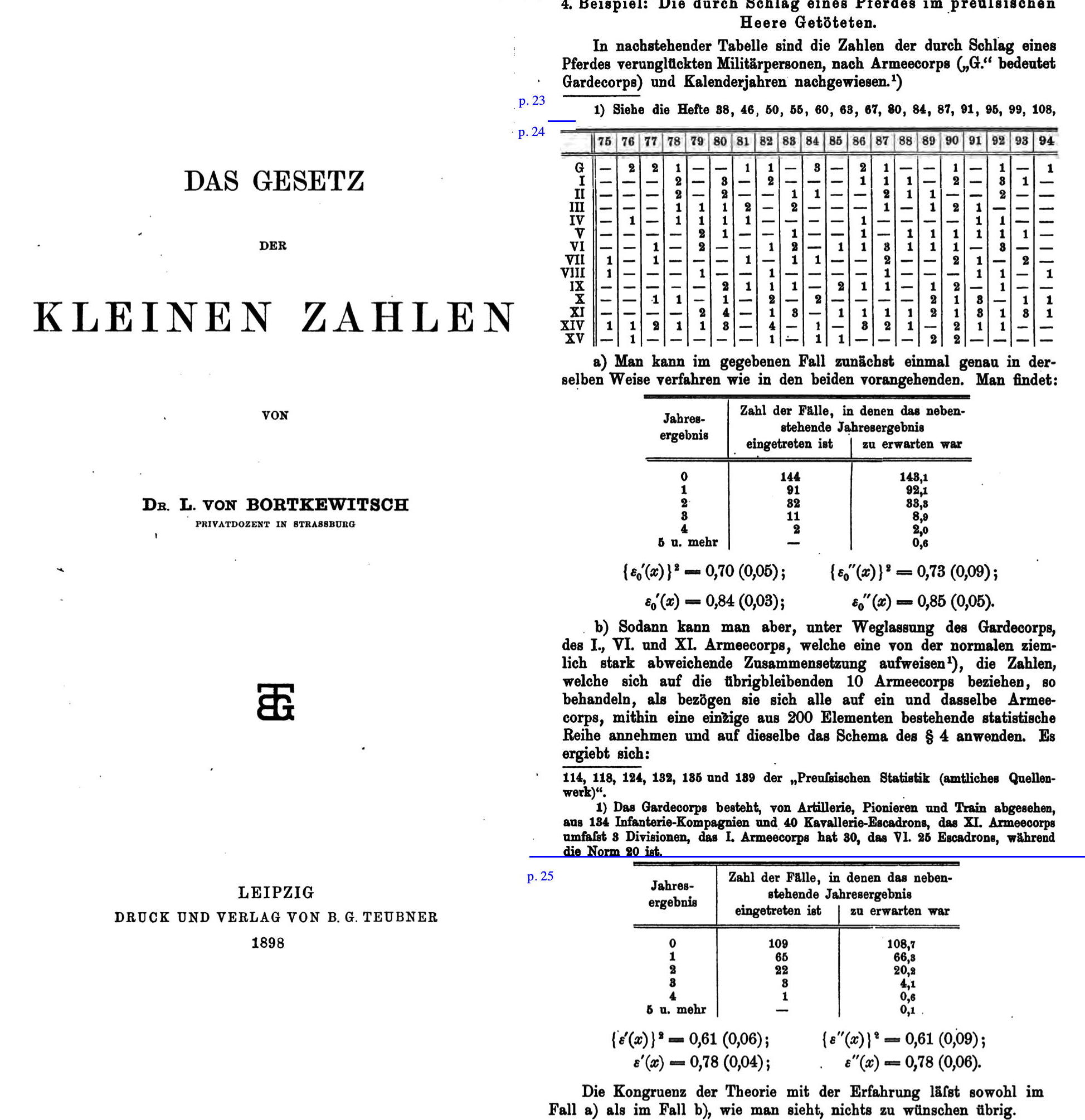
Figure 13.14: Section 12 of Bortkewitsch1898 book on the Poisson Distribution. The numbers

Example 5 V1 Flying-bomb hits in London, 1944

Example 6 Daily Births

Example 7 Monthly Deaths

Example 8 Daily car crashes

Does the Poisson Distribution apply to... ?

Yearly variations in numbers of killed in plane crashes?
Daily variations in numbers of births?
Daily variations in numbers of deaths [extra variation over the seasons]
Daily variations in numbers of traffic accidents [variation over the seasons, and days of week, and with weather etc.]
Daily variations in numbers of deaths in France in summer 2002 & 2003
Variations across cookies/pizzas in numbers of chocolate chips/olives.
Variations across days of year in numbers of deaths from sudden infant death syndrome. See

See

========

https://en.wikipedia.org/wiki/Normal_distribution#CITEREFStigler1982

dark https://physics.stackexchange.com/questions/28563/hours-of-light-per-day-based-on-latitude-longitude-formula

https://environhealthprevmed.biomedcentral.com/articles/10.1186/s12199-017-0637-4

car sppeds https://purr.purdue.edu/publications/2671/1

13.2.4 Normal

13.2.5 Hypergeometric

Non-Central Hypergeometric

13.2.6 Chi-square

===

EXERCISES

ADD YOUR OWN SEARCH RESULTS to table above

Hydroxychloroquine uniformity table.

few for differences

woolf

normal

transformations

13.3 Exercises

13.3.1 Clusters of Miscarriages [based on article by L Abenhaim]

Assume that:

15% of all pregnancies end in a recognized spontaneous abortion (miscarriage) -- this is probably a conservative estimate.
Across North America, there are 1,000 large companies. In each of them, 10 females who work all day with computer terminals become pregnant within the course of a year [the number who get pregnant would vary, but assume for the sake of this exercise that it is exactly 10 in each company]. *There is no relationship between working with computers and the risk of miscarriage.
a cluster'' of miscarriages is defined asat least 5 of 10 females in the same company suffering a miscarriage within a year''

Exercise: Calculate the number of 'clusters' of miscarriages one would expect in the 1,000 companies. Hint: begin with the probability of a cluster.

13.3.2 'Prone-ness' to Miscarriages ?

Some studies suggest that the chance of a pregnancy ending in a spontaneous abortion is approximately 30%.

On this basis, if a woman becomes pregnant 4 times, what does the binomial distribution give as her chance of having 0,1,2,3 or 4 spontaneous abortions?
On this basis, if 70 women each become pregnant 4 times, what number of them would you expect to suffer 0,1,2,3 or 4 spontaneous abortions? (Think of the answers in (i) as proportions of women).
Compare these theoretically expected numbers out of 70 with the following observed data on 70 women, each of whom had 4 pregnancies:

No. of spontaneous abortions:	0	1	2	3	4
No. of women with this many abortions:	23	28	7	6	6

Why don't the expected numbers agree very well with the observed numbers? i.e. which assumption(s) of the Binomial Distribution are possibly being violated? (Note that the overall rate of spontaneous abortions in the observed data is in fact 84 out of 280 pregnancies or 30%)

13.3.3 Automated Chemistries (from Ingelfinger et al)

At the Beth Israel Hospital in Boston, an automated clinical chemistry analyzer is used to give 18 routinely ordered chemical determinations on one order (glucose, BUN, creatinine, ..., iron). The ``normal'' values for these 18 tests were established by the concentrations of these chemicals in the sera of a large sample of healthy volunteers. The normal range was defined so that an average of 3% of the values found in these healthy subjects fell outside.

Using the binomial formula [even if it is na"{}ve to do so here], compute the probability that a healthy subject will have normal values on all 18 tests. Also calculate the probability of 2 or more abnormal values.
Which of the requirements for the binomial distribution are definitely satisfied, and which ones may not be?
Among 82 normal employees at the hospital, 52/82 (64%) had all normal tests, 19/82 (23%) had 1 abnormal test and 11/82 (13%) had 2 or more abnormal tests. Compare these observed percentages with the theoretical distribution obtained from calculations using the binomial distribution. Comment on the closeness of the fit.

13.3.4 Binomial or Opportunistic? (Capitalization on chance... multiple looks at data)

[Question from Ingelfinger et al. textbook] Mrs A has mild diabetes controlled by diet. Blood values vary rapidly, so think of each day as a new (independent) situation. Her morning urine sugar test is negative 80% of the time and positive (+) 20% of the time. [It is never graded higher than +].

At her regular visits to her physician, the physician always asks about last 5 days. At this particular visit, she tells the physician that the test has been + on each of the last 5 days.
What is the probability that this would occur if her condition has remained unchanged? Does this observation give reason to think that her condition has changed?
Is the situation different if she observes, between visits, that the test is positive on 5 successive days and phones to express her concern?

13.3.5 Can one influence the sex of a baby?

This question was prompted by this article in an 1979 issue of the New England Journal of Medicine.

Consider a binomial variable with $n = 145$ and $\pi = 0.528$. Calculate the SD of, and therefore a measure of the variation in, the proportions that one would observe in different samples of 145 if $\pi$ = 0.528. [In other words, the SD of the sampling distribution of the sample proportion.]

The following is abstracted from that NEJM article:

The baby's sex was studied in births to Jewish women who observed the orthodox ritual of sexual separation each month and who resumed intercourse within two days of ovulation. The proportion of male babies was 95/145 or 65.5% (!!) in the offspring of those women who resumed intercourse two days after ovulation (the overall percentage of male babies born to the 3658 women who had resumed intercourse within two days of ovulation [i.e. days -2, -1, 0, 1 and 2] was 52.8%).

How does the SD you calculated above help you judge the findings? And why did you not have to substitute the $p=0.655$ into the SD formula, and call it an SE of $p$?

13.3.6 It's the 3rd week of the course: it must be Binomial

In which of the following would $Y$ not have a Binomial distribution? Why?

The pool of potential jurors for a murder case contains 100 persons chosen at random from the adult residents of a large city. Each person in the pool is asked whether he or she opposes the death penalty; $Y$ is the number who say 'Yes.'
$Y$ = number of women listed in different random samples of size 20 from the 1990 directory of statisticians.
$Y$ = number of occasions, out of a randomly selected sample of 100 occasions during the year, in which you were indoors. (One might use this design to estimate what proportion of time you spend indoors)
$Y$ = number of months of the year in which it snows in Montreal.
$Y$ = Number, out of 60 occupants of 30 randomly chosen cars, wearing seatbelts.
$Y$ = Number, out of 60 occupants of 60 randomly chosen cars, wearing seatbelts.
$Y$ = Number, out of a department's 10 microcomputers and 4 printers, that are going to fail in their first year.
$Y$ = Number, out of simple random sample of 100 individuals, that are left-handed.
$Y$ = Number, out of 5000 randomly selected from mothers giving birth each month in Quebec, who will test HIV positive.
You observe the sex of the next 50 children born at a local hospital; $Y$ is the number of girls among them.
A couple decides to continue to have children until their first girl is born; $Y$ is the total number of children the couple has.
You want to know what percent of married people believe that mothers of young children should not be employed outside the home. You plan to interview 50 people, and for the sake of convenience you decide to interview both the husband and the wife in 25 married couples. The random variable $Y$ is the number among the 50 persons interviewed who think mothers should not be employed.

13.3.7 Tests of intuition

A coin will be tossed either 2 times or 20 times. You will win $2.00 if the number of heads is equal to the number of tails, no more and no less. Which is correct? (i) 2 tosses is better. (ii) 100 tosses is better. (iii) Both offer the same chance of winning.
Hospital A has 100 births a year, hospital B has 2500. In which hospital is it more that at least 55% of births in one year will be boys.

13.3.8 CI for proportion when observe 0/n or n/n

Oncologists often first try out new experimental agents on patients with metastatic disease who have failed all standard therapies. One (old) rule for deciding to abandon an experimental agent was: if it was tried on 14 successive patients, but did not show anti-tumour in any of them, i.e. if it `struck out' in all 14, yielding a response rate of 0/14.

Their reasoning is that this poor result ``rules out'' (with 95% confidence) the possibility that it would be active in more than 20% of future patients. In other words, the data are incompatible with any $\pi > 20\%.$

Check out their rule, by computing/obtaining a 95% 1-sided CI for $\pi.$

[Use a 1-sided CI if one is interested in putting just an bound on the probability of benefit or risk: e.g., what is upper bound on $= $ probability of getting HIV from HIV-infected dentist? See JAMA article ``If Nothing Goes Wrong, Is Everything All Right? Interpreting Zero Numerators'' by Hanley and Lippman-Hand

http://www.epi.mcgill.ca/hanley/Reprints/If\_Nothing\_Goes\_1983.pdf

and the rule of $3/n$' for a 1-sided 95\% CI. See also the second example (with sample size 4 !) in the sectionin defense of (some) small studies' in this article http://www.medicine.mcgill.ca/epidemiology/hanley/Reprints/Place\_of\_statistical\_1989.pdf

13.3.9 neg. correlations ... under-binomial variation

13.3.10 weights of offspring (pups/twins)

13.3.11 suicides

13.3.12 horsekicks

13.3.13 Visits to dentists (Cochran)

13.3.14 JH's steps per day

13.3.15 CD4 counts

13.3.16 tweets

13.3.17 accidents

13.3.18 bootstrap

13.3.19 no. of seats / doors / cyclinders in cars

13.3.20 sex ratio in accidents (FARS)

swedish twins reared together/apart Swedish Adoption/Twin Study on Aging (SATSA), 1984, 1987, 1990, 1993, 2004, 2007, and 2010 Nancy L. Pedersen Karolinska Institutet (Sweden)

Author(s)	PARAMETER	Statistic
Clayton and Hills	\(\pi\)	\(p = D/n\)
Moore and McCabe, Baldi and Moore	\(p\)	\(\hat{p} = y/n\)
Miettinen	\(P\)	\(p = y/n\)
This book	\(\pi\)	\(p = D/n\)

	r.v.	e.g.	E	S.D.
count:	\(y\)	2	\(n \times \pi\)	\(\{n \times \pi \times (1-\pi) \}^{1/2}\)
				i.e., \(n^{1/2} \times \sigma_{Bernoulli}\)

proportion:	\(p=y/n\)	0.2	\(\pi\)	\(\{\pi \times (1-\pi) / n \}^{1/2}\)
				i.e., \(\sigma_{Bernoulli} / n^{1/2}\)

percentage:	\(100p\%\)	20%	\(100 \times \pi\)	\(100 \times SD[p]\)