Chapter 3 Statistical Inference

The objectives of this chapter are to

• Understand what is meant by statistical inference

• Appreciate the fundamental difference between the Bayesian and Frequentist approaches

• In the Bayesian approach, the parameter is the subject of the statement. Statements are of the form: if, before observing the data, the parameter \(\theta\) was thought to have this probability distribution, then post-data, \(\theta\) should be thought of as having THIS probability distribution.

• In the Frequentist approach, the statements are indirect. They are (conditional) probabilistic statements about the data and about the performance of the procedure used to bracket parameter values. A variant ranks the possible parameter values according to how probable the observed data would be under each of these, but does not make direct probabilistic statements about the parameter values themselves.

• See several examples of both, and understood how the numerical results are arrived at

• Learn to be statisticallly/politically correct in interpreting these results

• Appreciate that in practice, the purely numerical differences between the results of the two approaches are often small.

Google gives the following definition for statistical inference

The theory, methods, and practice of forming judgments about the parameters of a population and the reliability of statistical relationships, typically on the basis of random sampling.

The Oxford English Dictionary defines it as

The drawing of inferences about a population based on data taken from a sample of that population; an inference drawn in this way; the branch of statistics concerned with this procedure.

Gelman and Hills start their regresssion textbook this way:

The goal of statistical inference for the sorts of parametric models that we use is to estimate underlying parameters and summarize our uncertainty in these estimates. We discuss inference more formally in Chapter 18; here it is enough to say that we typically understand a fitted model by plugging in estimates of its parameters, and then we consider the uncertainty in the parameter estimates when assessing how much we actually have learned from a given dataset. Gelman and Hills 2007.

We would add to these numerical statements about unknown (and unknowable) constants, as well as the mechanism or process that generated the limited data you got/get to observe.

David Cox begins his book Principles of Statistical Inference by taking the family of models as given and aims to:

1. give intervals or in general sets of values within which the parameter (or parameter set) is in some sense likely to lie;
2. assess the consistency of the data with a particular parameter value
3. predict as yet unobserved random variables from the same random system that generated the data;
4. use the data to choose one of a given set of decisions, requiring the specification of the consequences of various decisions.

He refers to the first two of these as interval estimation and measuring consistency with specified values of the parameter(s).

For orientation, before we get to parameters involved in multi-parameter regression models, here are some simple examples of parameters we might like to quantify probabilistically -- some scientific, some more personal or particularistic --

• Whether
• a potential hemophilia carrier is in fact a carrier
• a particular email is malicious
• a person committed the crime they are accused of

• a person has been infected with a certain virus

• The proportion of
• thumbtacks that land on their back when tossed
• your time that you are being productive
• the earth's surface that is covered by water
• your driving time that you are on the phone
• your time (over the entire year) that you spend inside
• patients whose disease would respond to a medication

• people who would volunteer for a demanding survey or long-term research study

• The numerical value for
• the density of the Earth,relative to water
• the age of a person whom you have just met
• your cholesterol level
• the mean depth of the ocean
• the 20th percentile of the depths of the ocean

• the median age of a population

To address the uncertainties involved in the judgements/inferences, some use of probabilities is required.

When considering the first objective, namely providing intervals or sets of values likely in some sense to contain the parameter of interest, Cox tells us

There are two broad approaches, called frequentist and Bayesian, respectively, both with variants. Alternatively the former approach may be said to be based on sampling theory and an older term for the latter is that it uses inverse probability.

In their preamble to their chapter on inferemce, Clayton and Hills tell us that

There are two radically different approaches to associating a probability with a range of parameter values, reflecting a deep philosophical division amongst mathematicians and scientists about the nature of probability. We shall start with the more orthodox view within biomedical science.

Clayton and Hills completed their book in 1993. Since then, propelled by greater computer power, and by people like Clayton's Cambridge colleague David Spiegelhalter, whose book we will start with, the Bayesian approach to 'associating a probability with a range of parameter values' has become more common. It has not yet reached the status of 'customary or conventional, as a means or method; established.' that the dictionaries give as the meaning of orthodox. In any case, we should not take Clayton and Hills' use of the phrase 'more orthodox' to describe the frequentist approach to mean that the Bayesian approach 'does not conform to the approved form of analysis' or is in some sense 'wrong.'

The first-established of the two 'schools' (or 'churches') of statistical inference** makes direct probabilistic statements about the possible parameter values. This approach goes back at least as far as the mid-1700's essay 'A method of calculating the exact probability of all conclusions based on induction'; ironically the author was a Presbyterian minister.

The developments since then are nicely told in the very readable book The Theory That Would Not Die: How Bayes' Rule Cracked the Enigma Code, Hunted Down Russian Submarines, and Emerged Triumphant from Two Centuries of Controversy by Sharon Bertsch McGrayne, and in her Microsoft lecture and her Google lecture.

Maybe, by calling it the more 'orthodox', all that Clayton and Hills mean is that the frequentist approach is more popular method today. It got a slow start, and dates from the early 20th century. (In one of our sampling exercises, we will try to determine the relative frequencies of the two approaches in the epidemiology and medical literature).

Interestingly, if you use Google Books Ngram Viewer you get a different sense. Maybe this is because the majority don't need to justify the methods they use!

Frequentist statements are indirect. They are (conditional) probabilistic statements about the data and about the performance of the procedure used to bracket the parameter values. A variant on it ranks the various possible parameter values according to how probable the observed data would be under each of these, but does not make direct probabilistic statements about the parameter values themselves. Because it is indirect, conditional, the results are often interpreted incorrectly.

We begin with the direct method, one that studies tell us we are born with, and use throughout our lives, both consciously and subconsciously, to continue to learn/update.

When we learn a new motor skill, such as playing an approaching tennis ball, both our sensors and the task possess variability. [...] We show that subjects internally represent both the statistical distribution of the task and their sensory uncertainty, combining them in a manner consistent with a performance-optimizing bayesian process. The central nervous system therefore employs probabilistic models during sensorimotor learning. Bayesian integration in sensorimotor learning

leading to this New York Times headline

Subconsciously, Athletes May Play Like Statisticians

3.1 The Bayesian Approach

to probability statements concerning parameter values.

Bayesian inference refers to statistical procedures that model unknown parameters [...] as random variables. [...] Bayesian inference starts with a prior distribution on the unknown parameters and updates this with the likelihood of the data, yielding a posterior distribution which is used for inferences and predictions. Gelman and Hills, 2007, page 143.

This paragraph, taken from this chapter An Overview of the Bayesian Approach in the book Bayesian Approaches to Clinical Trials and Health-Care Evaluation by David Speigelhalter et al, describes it well:

The standard interpretation of probability describes long-run properties of repeated random events (Section 2.1.1). This is known as the frequency interpretation of probability, and standard statistical methods are sometimes referred to as 'frequentist'. In contrast, the Bayesian approach rests on an essentially 'subjective' interpretation of probability, which is allowed to express generic uncertainty or 'degree of belief' about any unknown but potentially observable quantity, whether or not it is one of a number of repeatable experiments. For example, it is quite reasonable from a subjective perspective to think of a probability of the event 'Earth will be openly visited by aliens in the next ten years', whereas it may be difficult to interpret this potential event as part of a 'long-run' series. Methods of assessing subjective probabilities and probability distributions will be discussed in Section 5.2.

Section 3.1 SUBJECTIVITY AND CONTEXT emphasizes that 'the vital point of the subjective interpretation is that Your probability for an event is a property of Your relationship to that event, and not an objective property of the event itself.' Moreover, 'pedantically speaking, one should always refer to probabilities for events rather than probabilities of events, and the conditioning context used in Section 2.1.1 includes the observer and all their background knowledge and assumptions.'

That there is 'always a context' goes along with what we read in Alan Turing's recently de-classified essay The Applications of Probability to Cryptography. Under section 1.2 ('Meaning of probability and odds') he starts out

I shall not attempt to give a systematic account of the theory of probability, but it may be worth while to define shortly probability and odds. The probability of an event on certain evidence is the proportion of cases in which that event may be expected to happen given that evidence. For instance if it is known the 20% of men live to the age of 70, then knowing of Hitler only Hitler is a man we can say that the probability of Hitler living to the age of 70 is 0.2. Suppose that we know that Hitler is now of age 52 the probability will be quite different, say 0.5, because 50% of men of 52 live to 70.

Not all context is subjective. We will start with a context where the initial (starting out, pre-new-data) probability is objective.

Just before we do, we include this passage from Clayton and Hills, in subchapter 10.2 Subjective probablity, which they denote as optional material.

The second approach to the problem of assigning a probability to a range of values for a parameter is based on the philosophical position that probability is a subjective measure of ignorance. The investigator uses probability as a measure of subjective degree of belief in the different values which the parameter might take. With this view it is perfectly logical to say that there is a probability of 0.9 that the parameter lies within a stated range.
Before observing the data, the investigator will have certain beliefs about the parameter value and these can be measured by a priori probabilities. Because they are subjective every scientist would be permitted to give different probabilities to different parameter values. However, the idea of scientific objectivity is not completely rejected. In this approach objectivity lies in the rule used to modify the a priori probabilities in the light of the data from the study. This is Bayes' rule and statisticians who take this philosophical position call themselves Bayesians.
Bayes' rule was described in Chapter 2, where it was used to calcu- late the probabilities of exposure given outcome from the probabilities of outcome given exposure. Once we are prepared to assign probabilities to parameter values, Bayes' rule can be used to calculate the probability of each value of a parameter (\(\theta\)) given the data, from the probability of the data given the value of the parameter.
The argument is illustrated by two tree diagrams. Fig. 10.2 illustrates the direction in which probabilities are specified in the statistical model — given the choice of the value of the parameter, \(\theta\), the model tells us the probability of the data. The probability of any particular combination of data and parameter value is then the product of the probability of the parameter value and the probability of data given the parameter value. In this product, the first term, Pr(\(\theta\)), represents the a priori degree of belief for the value of \(\theta\) and the second term, Pr(Data | \(\theta\) ), is the likelihood. Fig. 10.3 reverses the conditioning argument, and expresses the joint probabilityas the product of the overall probability of the data multiplied by the probability of the parameter given the data. This latter term, Pr( \(\theta\) | Data), represents the posterior degree of belief in the parameter value once the data have been observed. Since the joint probability of data and parameter value is the same no matter which way we argue, so that \[Pr(\theta) \times Pr(Data | \theta) = Pr(Data) \times Pr(\theta | Data),\] so that \[Pr(\theta | Data) = \frac{Pr(\theta) \times Pr(Data | \theta)}{Pr(Data)}\] Thus elementary probability theory tells us how prior beliefs about the value of a parameter should be modified after the observation of data.

Their 2 figures nicely show that the difference is in the directionality or conditioning, i.e. is the object \[Pr(\theta | data) \ \ \ OR \ \ \ Pr(data | \theta) \ \ ?\]

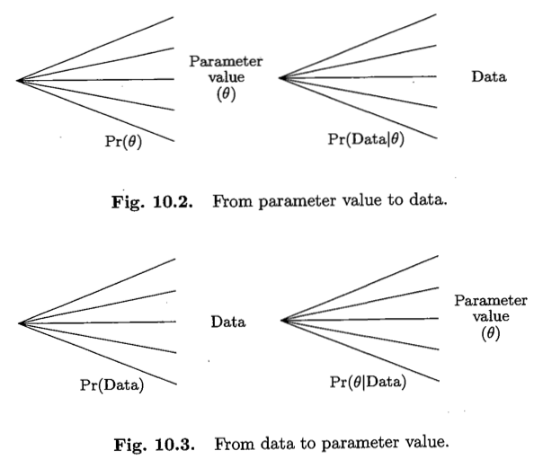
Figure 3.1: From Chapter 10.2 of Clayton and Hills

Without getting into the details of the calculations, we will apply the Bayesian approach to the first example in each of the parameter genres listed above. The point is to illustrate how direct and unambigous the answer is in each case. To avoid being distracted by the details, you might wish to skip the detailed mathematical calculations involved, as well as the asides/tangents.

3.1.1 Example: parameter is 2-valued: yes or no

In the first genre, the parameter is personal or particular. In each of the examples, the true state is binary. The potential hemophilia carrier is a hemophia carrier or is not; the particular email is either malicious or is not; the person in question either committed the crime ot did not. So, there are just two possible parameter values: yes or no, is or is not.

From the outset, just like in Turing's example, there is a given context. For example, suppose a woman's brother is known to have haemophilia.

hemophilia: a medical condition in which the ability of the blood to clot is severely reduced, causing the sufferer to bleed severely from even a slight injury. The condition is typically caused by a hereditary lack of a coagulation factor, caused by a mutation in one of the genes located on the X chromosome. - Google

Just knowing this, the probability that the woman is a hemophilia carrier is 50% or 1/2.

Today, genetic testing of the carrier can help determine whether the woman is a carrier. But when JH first taught 607, the only time to learn more about her carrier status (and move her probability to 1, or towards 0) was after the births of her sons: their status was knowable virtually immedediately.

If it is determined that the first son has hemophilia, it establishes that she IS a carrier, thereby moving the probability up to 1. If he does not, it moves the probability down to 1/3: in other words, among 'women like her', i.e, potential carriers who also have had 1 son who turned out to be Normal (NL), 1/3 of the sons are the sons of carriers, and 2/3 are the sons of non-carriers.

The continued updating as the women with a NL son gave birth to a second son, and so on, is shown in the diagram below, with C used as shorthand for 'Is a Carrier.' Technically speaking, each sequential P[C] should indicate that it is 'conditioned on' -- and thus reflects the information in -- the history up to that point. In other words, the 1/5 probability refers to P[C | both sons are NL], where "|" stands for 'given that', or -- to use Turing's phrase -- 'on the evidence that'.

Figure 3.2: At the outset, each woman had a 50:50 chance of being a haemophilia carrier. Accumulating information from the hemophilia status of the sons increasingly 'sorts' or segregates the women by moving their probabilities of being a carrier TO 1 (100%) or FURTHER TOWARDS 0 (0%). It 'updates' the probablity of being a carrier, P[C]. For brevity, the ' | data' in each P[C | data] is omitted.

Before moving on the the next type of parameter, a few points

• In the hemophilia (and if interested, the transgenic mice) example, the 'starting' probability is objective and the post-data probabilities have a 'long-run' or 'in large numbers of similar instances' interpretation. One could make a diagram that shows the expected numbers 'in every 100 women like this.'

• There is nothing special about the 'starting out' probability P[C] of 0.5. Before a pregnancy test, or a pre-natal diagnostic test, for example, the probability of the target Condition/state of interest/concern would be a function of many other factors, and could in theory take on any value between 0 and 1. The (starting out, pre-filter) proportion of malicious emails would depend on which of a person's email accounts it was.

• In the language of diagnostic tests, each 'Son as a test of the mother's carrier status' has 50% sensitivity and 100% 'specificity'. For sensitivity, this puts it on par with the Pap test for cervical cancer: the main problem withe latter is in the sampling. For specificity, it is better than most tests.

• The shiny app From Pre-test to Post-test Probabilities shows how the initial average (pre-test) probability is segregated into 2 post-test probabilities by the 2 possible test results, and the role of the 2 error-probabilities (just about all tests are fallible) in how well they push them out.

• The 'starting out' probability could be subjective. For example it could be one's impression (before getting to see up close how wrinkled their face is) as whether the person is a smoker, or one's assessment of the probability that the accused is guilty (before getting to hear the DNA expert, or lie detection report) based on how credible the accused appears to be, and all of the other evidence to date.

• The posterior distribution for the parameter merges (adds) two sources of information.

• But the focus is less on where we start, and more on how much we have learned from the new data.

Bayes' rule: Guide (at several levels)

ref: https://arbital.com/p/bayes_rule/?l=1zq

3.1.2 Example: parameter is a proportion

In theory, in this genre, the true parameter value could in theory lie anywhere between 0 and 1, But again, just like in Turing's example, we seldom start from complete ignorance, or with -- in the title of pscychologist Stephen Pinker's book -- a blank slate. Even if you have never seen thumbtacks tossed onto on a surface, you can reason informally, and indicate what proportions are unlikely and likely, and where along the (0,1) scale you would 'put your money'.

You could do the same when asked what proportions of your time that you are being productive, or on the phone, or sedentary, or indoors. Mind you, you might be 'way off' with your claims, but the nice thing is that --- and this is the point of this course -- you can generate data to narrow down the true proportion.

The other nice thing with the Bayesian approach in particular is that -- no matter whether you believe the proportion is low or medium or high, we can work out what your post-data beliefs should be. It is a matter of mathematics. If, before collecting any new data, we have 'no idea' -- a common phrase among todays's generation, one that, if it is uttered with empahsis on the 'no', irks JH to no end -- what the true parameter value is, that is easily handled. Moreover, enough valid data will (or should!) trump the pre-data beliefs.

On a side note: Dick Pound, a former chancellor of McGill University, and first president of the World Anti-Doping Agency is a staunch advocate of strict drug testing for athletes. Discussing the National Hockey League in November 2005, Pound said, 'you wouldn’t be far wrong if you said a third of hockey players are gaining some pharmaceutical assistance.' Pound would later admit that he completely invented the figure. Both the NHL and NHLPA have denied the claims, demanding Pound provide evidence rather than make what they term unsubstantiated claims. Since his comments were made, some NHL players have tested positive for banned substances, including Bryan Berard, José Théodore, and two of 250 players involved in Olympic testing. As of June 2006, there had been 1,406 tests in the program jointly administered by the league and the union, and none has come up with banned substances under NHL rules. Pound remained skeptical, claiming the NHL rules were too lax and unclear, as they do not test for some banned substance, including certain stimulants. In an interview with hockey blogger, B. D. Gallof, of Hockeybuzz on December 19, 2007, Pound was asked to expand on the 30% comment and subsequent reaction, expounded that stimulants was 'the NHL's drug of choice'. He also cited that the NHL will have no credibility on a drug policy if it, and other sports, continue to run things 'in-house'. https://en.wikipedia.org/wiki/Dick_Pound and https://www.cbc.ca/sports/hockey/dick-pound-slams-nhl-s-drug-policy-1.557993

Even before studying/asking them, investigators would have some sense of the proportions of patients whose disease would respond to a medication, or people who would volunteer for a survey or research study. These iimpressions would probably be based on previous analogous situations, and the 'literature', but would vary from pundit to pundit. But ultimately, they could be much improved and narrowed (and even replaced entirely) by new-data-based ones.

The proportion of the earth's surface that is covered by water is easy to determine: just look up a reputable source. But what if you weren't able to, but did have access to the database of 933 million recordings in the SRTM30PLUS database. It has altitude/depth measurements for 43,200 x 21,600 = 933,120,000 locations. This database is so large that you would have to sample from it. From a thousand randomly chosen loactions, you would be able to 'trust' the first decimal in your estimate; from a million you should be able to trust the second -- and maybe the third.

Since we already know/remember from high school 'roughly' what the proportion is, we will leave it for an exercsie in another chapter. In this chapter, following the advice of master-teacher Fred Mosteller, we use examples where the correct answer is not known with any precision. The proportion of these we probably know the least about is the thumbtack one. However, it has fewer personal benefits than knowing what proportion of your time you are being productive. Moreover, we have a nice written account of how you might go about learning this personal proportion.

Worked example (productivity)

In his book Elementary Bayesian Statistics, Gordon Antelman informally introduces and illustrate a Bayesian analysis of an uncertain proportion with a slightly modified version of a novel and useful application of work sampling discussed by Fuller (1985). We have changed his notation for the proportion of your time spent in productive work, and called it \(\pi\), and also modified some of his words.

Suppose you, as a good up-to-date manager practicing continuous quality and productivity improvement, have some ideas on improving your own productivity. To see if these ideas have any merit, you would like to compare some 'before' measure of productivity with a comparable 'after' measure of productivity.
For now — we shall come back to this example several times — let us focus on just a 'before' measure. The measure to be used is the proportion of your time spent in productive work, call it \(\pi\), as opposed to time spent doing something that would not have needed doing if things had been done right the first time. Examples of the latter might include searching for a misplaced document, recreating a deleted computer file, following up on a customer's complaint, or waiting past a scheduled time for a meeting to start. [Today, we would add being on social media, or browsing the web for non-work-related matters] Rather than saying \(\pi\) is not (precisely) 'known', it is better to say that '\(\pi\) is uncertain'; from your job experience, you would really know quite a lot about p. For example, you might be almost certain that it is greater than 0.50, less than 0.90, and you might assess your odds that \(\pi\) is between, say, 0.60 and 0.80 to be about 9 to 1. A precise statement of these beliefs will be your prior distribution for \(\pi\).
You would probably feel uncomfortable — most people do — about assessing this prior distribution, especially since there are an infinite number of states; viz., all of the values between zero and one. But, without any real loss, you can bypass the infinite-number problem by rounding the values of \(\pi\) to the nearest 5% or 10%, making the problem discrete. Then you have a contemplatable Bayes' theorem, like those discussed in Chapter 4, with the finitely many \(\pi\)-values as the possible "states". (When we reconsider this example later in this chapter, you will see that, with a little theory, the infinite number of \(\pi\)-values can almost always be handled very neatly and more easily.)

PRIOR BELIEFS For illustration, he supposes you choose just five possible values for \(\pi\), and assess your prior distribution. Since R does not allow Greek symbols, we will refer to it by uppercase P and assess your prior distribution. This possible prior distribution, shown below, would reflect, for example, that your judgment is that there is only about one chance in 20 that \(\pi\) rounds to 0.50, about one chance in 20 that \(\pi\) rounds to 0.90, about one chance in four that it rounds to 0.60, a little more than one chance in three that it rounds to 0.70, and a little less than one chance in three that it rounds to 0.80.

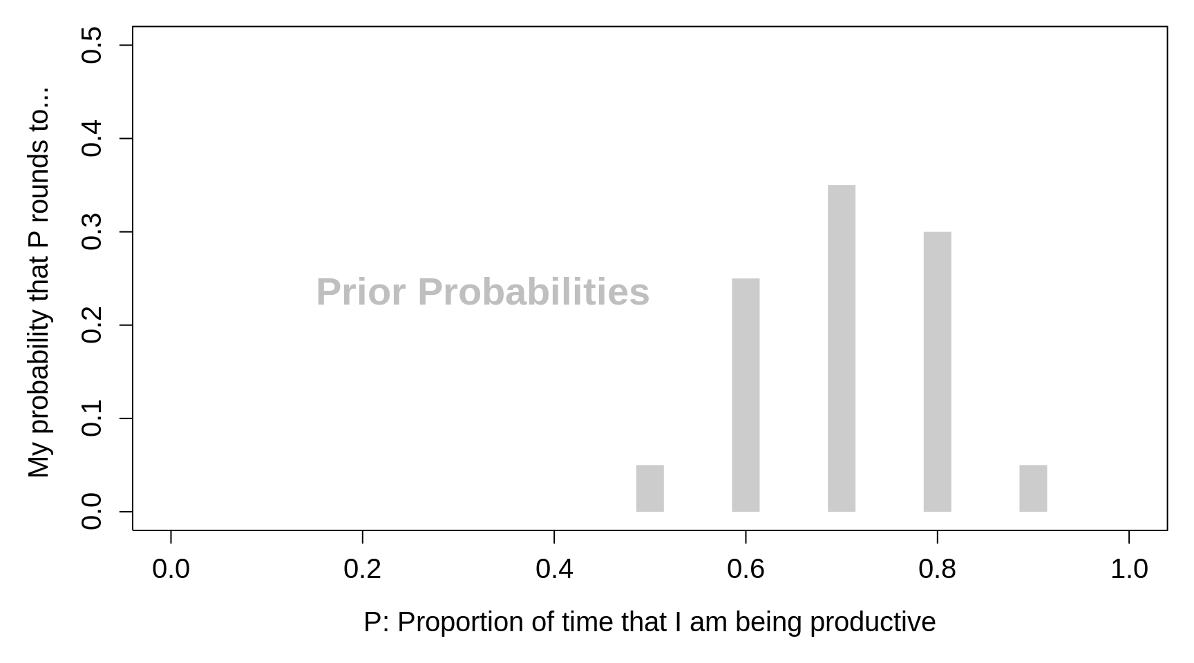
Figure 3.3: Prior Probabilities for the parameter P, the proportion of time that I am being productive.

DATA: Suppose you are fitted with a beeper set to beep at random times; when the beeper beeps, you classify the task being worked on as W — for 'productive Work', or F — for 'Fixing' (or today we mght say 'Fiddling' or 'Fooling around' or wasting time).

Although we will skip the technicalities, it is important that the experiment be designed so that the trials are independent. Beeps should be unpredictable so you do not arrange, possibly subconsciously, to be doing productive work at the beep. They probably also should not be too close together to make the independence assumption more reasonable.

Suppose the first four trials give the data \(F_1, F_2, W_3\), and \(F_4\).

Below is a picture showing the effects of the data FFWF on the prior distribution. Three F's in four trials increase your probabilities for the two smaller values of P and decrease your probabilities for the three larger ones.

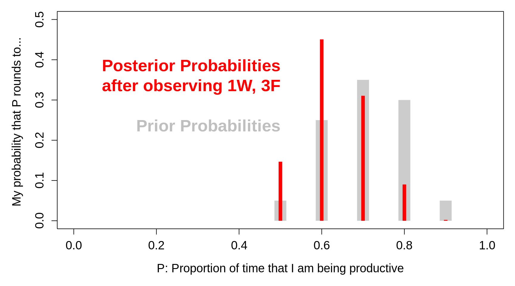
Figure 3.4: Prior Probabilities for the parameter P, the proportion of time that I am being productive, together with the corresponding posterior probabilities, after observing that in n = 4 randomly sampled occasions, I was actually productive in only 1 of the 4.

The sample alone most strongly supports a value for P of 0.25 (one W in four trials); had the prior included a value of P of 0.25, the (relative) increase in going from prior to posterior would have been greatest for that value.

For the assumed prior, in which only p's of 0.50, 0.60, 0.70, 0.80, or 0.90 are considered, the sample evidence FFWF in favor of a P near 0.25 can only push up the posterior probabilities for the nearest possible values - 0.50 and 0.60. (The seemingly harder consideration of all possible p's between zero and one will handle this kind of situation more logically.)

Below we show the 'continuous P ' version Antelman refers to. To make this, we calculated the mean and variance of his discrete (5-point) prior distribution, and converted them to the 2 parameters, \(a\) and \(b\), of the beta distribution with the same mean and variance.

Conveniently, the posterior density is also a beta distribution, but with parameters \(a+1\) and \(b+3\).

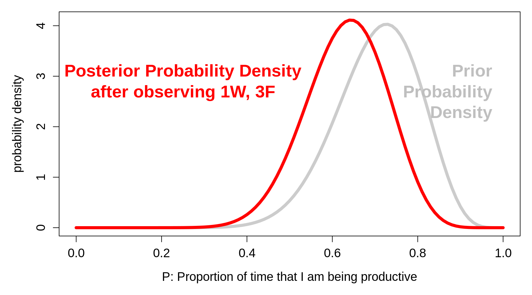
Figure 3.5: Prior probability densities for the parameter P, the proportion of time that I am being productive, together with the corresponding posterior densities, after observing that in n = 4 randomly sampled occasions, I was actually productive (W) in only 1 of the 4.

Before moving on the the next type of parameter, a few points:

• The beta distribution nicely shows how the prior information/impression and the new data get combined. The \(a\) and \(b\) parameters of the prior distribution are 14.8 and 6.2. Together, they determine the mean, \(a/(a+b)\), the median, the mode, \((a-1)/(a+b-2)\), and the variance, \(mean(1-mean)/(a+b+1)\) of the prior distribution. Their conterparts in the data-likelihood are 1 and 3. The '\(a\)' and '\(b\)' parameters of the posterior distribution are 15.8 and 9.2: the \(a\)'s add, and the \(b\)'s add. In other words, the distribution of one's pre-data beliefs is the distribution one would have after 'seeing' 14.8 W's and 6.2 F's; the distribution of one's post-data beliefs is the distribution one would have after 'seeing' 15.8 W's and 9.2 F's. The (synthetic) experience-equivalent of the numbers of Ws and F's in the prior are added to the actual (observed) numbers of Ws and F's in the data to arrive at the (new) posterior distribution.

• You are probably wondering what the posterior distribution would look like with more data. Here is what it would look like after observing 7 out of 25 or 13 out of 25. The modes of the posterior distributions are still somewhat influenced by the prior -- as they are still well above P=7/25 = 0.28 and P=13/25 = 0.52. If the data were 70/250 or 13/250, the modes would be closer to P= 0.28 or P = 0.52; in other words, the data would 'swamp' -- or 'trump' -- the prior.

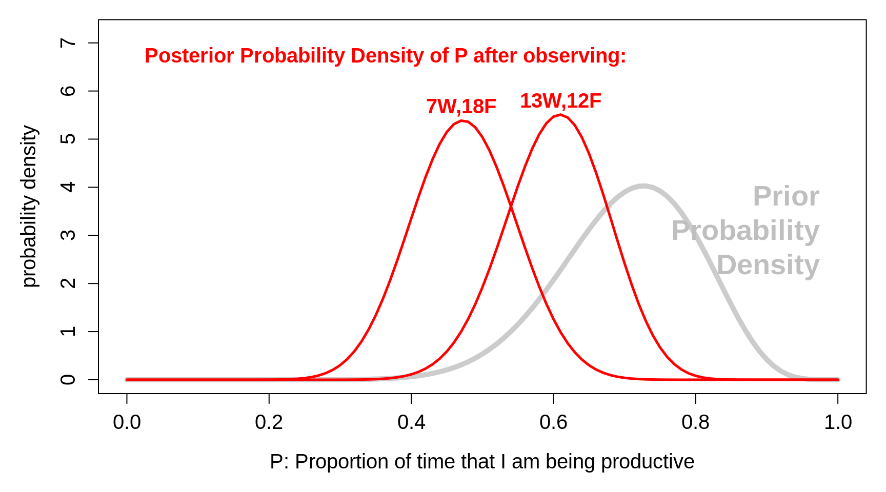
Figure 3.6: Prior probability densities for the parameter P, the proportion of time that I am being productive, together with the corresponding posterior densities, after observing that in n = 25 randomly sampled occasions, I was actually productive (W) in only 7 of the 25, or 13 of the 25.

• Be thinking about your prior for the proportion of thumbtacks that land on their back, and the proportion of the Earth's surface that is covered by water, or [these words written on March 30, 2020, before any trial data] the proportion of patients with mild symptoms of covid-19 who would benefit from chloroquine.

• Think about how you might elicit a prior distribution. You might want to Google 'tools for eliciting prior distributions' -- or consult Chapter 5 of Spiegelhalter's book.

We now move on to last parameter genre we will consider.

3.1.3 Examples: parameter is a personal number or population mean

We will start with a discrete version of a commonly-wondered-about parameter, the age of a person whom you have just met, or seen a photo of. We will then go on to full numerical examples: your average cholesterol or blood pressure level, a baseball player's batting average

Example 1

How old (or what age -- if you prefer to avoid speaking of 'old') do you think this IBC2006 attendee was when this photo was taken? This is the parameter of interest.

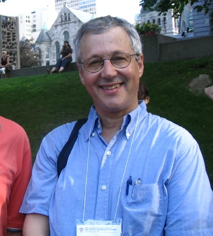
Figure 3.7: An attendee at the International Biometrics Conference, held at McGill in July 2006

He tells you he got his PhD 32 years earlier. Based on the distribution of ages at which people get their PhD (shown in grey below), that puts his current age somewhere in the blue distribution.

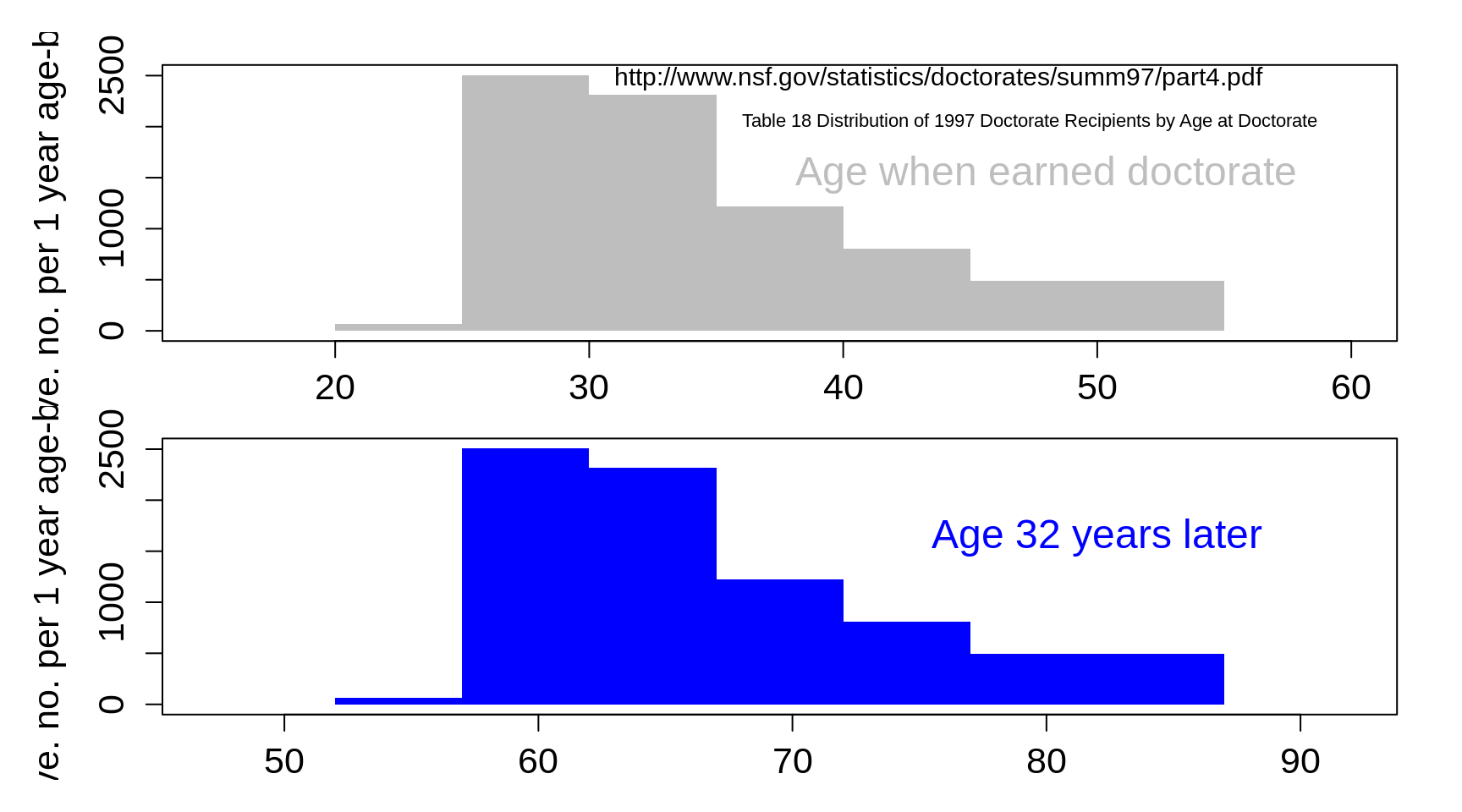
Figure 3.8: Current ages of persons who obtained PhD 32 years earlier.

This is a somewhat unusual example, as the blue distribution is very wide -- partly because we could not find age-at-graduation data specific to PhD graduates in statistics in 1974. We suspect that that specific distribution is a good deal narrower than the one shown. In the next chapter, you will see that other indirect measures of age are a good bit tighter than this.

Nevertheless, it emphasizes that, depending on what impression you got form the photo alone, you may now wish to revise your estimate of the person's age. We suspect that many of you would have initially though he looks like he was in mid 50s, and so would have made guesses like those shown in red in the top panel. If you are one of those, then you will want to revise the age upwards, as we do in the green in the bottom panel.

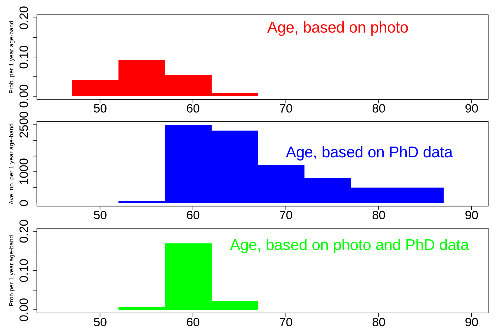
Figure 3.9: If he looked like he was in mid 50s

If you initially thought he looked like he was 'around 60' you would have made guesses like those shown in red in the top panel. If you did, then you will want to revise upwards a little, as is shown in green, and now put hime him somewhere around 60, or a bit above.

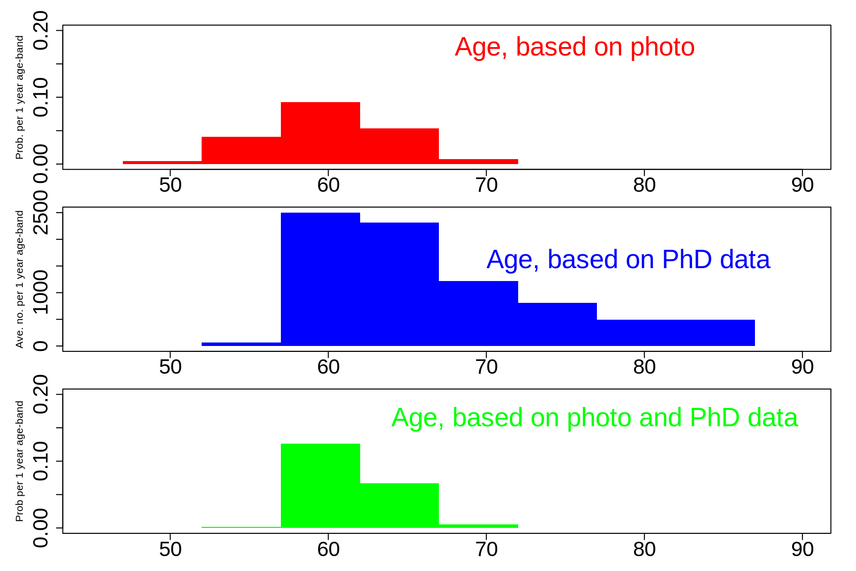
Figure 3.10: If If he looked like he was around 60.

If you initially thought he looked like he was 'in his mid 60s' your estimate is more in line with the age-at-PhD data, and so you would not revise as much. You might bet a bit more on the 'around 60' age-bracket.

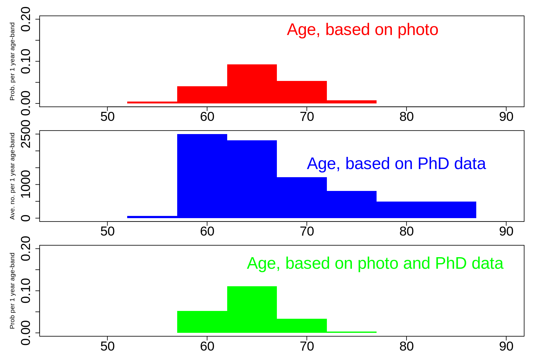
Figure 3.11: If If he looked like he was in his mid 60s.

As we noted, the PhD data have too much of a right tail, and so it is driving up the estimates. If you are now curious as how keen your 'age-estimation' skills are, here is a link to the Google Scholar page of the statistician whose age we have been trying to determine.

Age estimation via face images (image-based age estimation) is a growing research area, with many possible applications.

We now describe 2 more classical examples

Example 2

Spiegelhalter et al. address this in their Example 3.4: 'Suppose we are interested in the long-term systolic blood pressure (SBP) in mmHg of a particular 60-year-old female.'

We take two independent readings 6 weeks apart, and their mean is 130. We know that SBP is measured with a standard deviation \(\sigma = 5.\) What should we estimate her SBP to be?

They then go on to give the frequentist ('standard', 'orthodox') 95% confidence interval, of 123.1 to 136.9, centered on the measured value of 130 [we will come later to how they calculated this]. They continue, ...

However, we may have considerable additional information about SBPs which we can express as a prior distribution. Suppose that a survey in the same population revealed that females aged 60 had a mean long-term SBP of 120 with standard deviation 10. This population distribution can be considered as a prior distribution for the specific individual.

The posterior distribution, computed from the combination of the 130 measured on the woman, and the prior, is centered on 128.9 and the 95% interval is 122.4 to 135.4.

This posterior distribution reveals some 'shrinkage' towards the population mean, and a small increase in precision from not using the data alone.
Intuitively, we can say that the woman has somewhat higher measurements than we would expect for someone her age, and hence we slightly adjust our estimate to allow for the possibility that her two measureshappened by chance to be on the high side. As additional measures are made, this possibility becomes less plausible and the prior knowledge will be systematically downgraded.

Before going on to example 3, we emphasize that the 128.9 is a compromize between the personal mean of 130, and the (prior) poulation mean of 120: it is a weighted average, with (relative) weights that are the reciprocals of the squares of the 2 standard deviations, the reciprocals of \(\frac{5^2}{2}\) and \(10^2,\) i.e., \(\frac{2}{25} = 0.08\) and \(\frac{1}{10^2} = 0.01.\) The 128.9 is 8/9ths closer to the measured 130 than it is to the population mean of 120. It is slightly 'shrunk' toawards the population. This is why physicians might not believe that the 130 is correct, and might ask for more measurements before putting this woman on blood pressure-lowering drugs.

[The already cited 'Bayesian integration in sensorimotor learning' illustrates how as humans, we automatically combine estimates of different precisions into one more precise estimate, and do so using the same mathematical laws that are used in the Bayesian approach!]

Example 3

One article that does go into some detail about a similar situation is the very nice medically-useful – and didactic article Estimating an Individual’s True Cholesterol Level and Response to Intervention by Les Irwig, Paul Glasziou, Andrew Wilson and Petra Macaskill.

It begins with a single measurement, before dealing with an average of several measurements on the same person. It also gives separate charts for persons of different ages, and deals not just with point and interval estimates, but also derives probability statements for the possibility that the person’s true cholesterol is above some threshold that should trigger intervention. The appendix is a nice tutorial for combining information.

Their abstract begins:

An individual’s blood cholesterol measurement may differ from the true level because of short-term biological and technical measurement variability. Using data on the within-individual and population variance of serum cholesterol, we addressed the following clinical concerns: Given a cholesterol measurement, what is the individual’s likely true level? The confidence interval for the true level is wide and asymmetrical around extreme measurements because of regres-sion to the mean. Of particular concern is the misclassification of people with a screening measurement below 5.2 mmol/L who may be advised that their cholesterol level is 'desirable' when their true level warrants further action.

The first half of the paper, which deals with two related topics, (a) Estimating the True Cholesterol Level, and (b) assesing the Probability of Misclassification shows the primary elements, and these notes will focus on the highlights. [after these, extensive excerpts will be included]

The results for (a) and (b) were presented as 2 Figures. The first gave the (posterior) credible interval for a person’s true cholesterol level based on either 1, or an average of 3, measurements, using on the horizontal axis the measured value, and on the vertical one the point and 95% credible interval. Using a graph (rather than a formula) allows the clinician to use it for all possible ‘what if’s.

Below, we will illustrate it using one specific example, a person whose measured value was 7.15.

The second uses the (posterior) credible interval to calculate the probability that someone with a specific measured value has a true level that is above a certain threshold level used in treatment guidelines. Thus, the key tool is the posterior distribution itself, and so we give the statistical basis for this.

Reasons to take a Bayesian approach

The reason this problem arises in the first place is because of short term biological variability in the quantity of interest in the person in question. If we were measuring a person’s height, we could do so carefully at just one time-point: it would not be different a week or month from now; it remains quite stable over several years. [it does vary slightly over the day, but, be keep it simple, we could speak of one’s height at mid-day]. The same is not the case for a person’s cholesterol level: even if we measured it very carefully at one time, it would be genuinely different a week or month later, even in the absence of any intervention of lifestyle change. (The same applies, more strikingly, for other blood levels such as C-reactive protein (CRP), which is a marker of inflammation).

Thus any single measurement, or any average of a finite number of determinations, is imprecise. So what’s new? Don’t we meet this issue all the time in statistics?

The point of Irwig's article is that we should not rely solely on the estimate based on the person’s measurements, but rather should combine it with an estimate based on outside information.

The same reasoning is at work when a physician repeats a measurement that seems extreme. In so doing, (s)he is not relying only on the point or interval estimate provided by the measurement itself: rather (s)he is also using knowledge of how this measurement behaves in other similar persons! And what we know about others, even if collectively, can help us with an individual.

All of the technical details are available in these notes, prepared for bios601 Here we will skip to the 'botom line' diagrams.

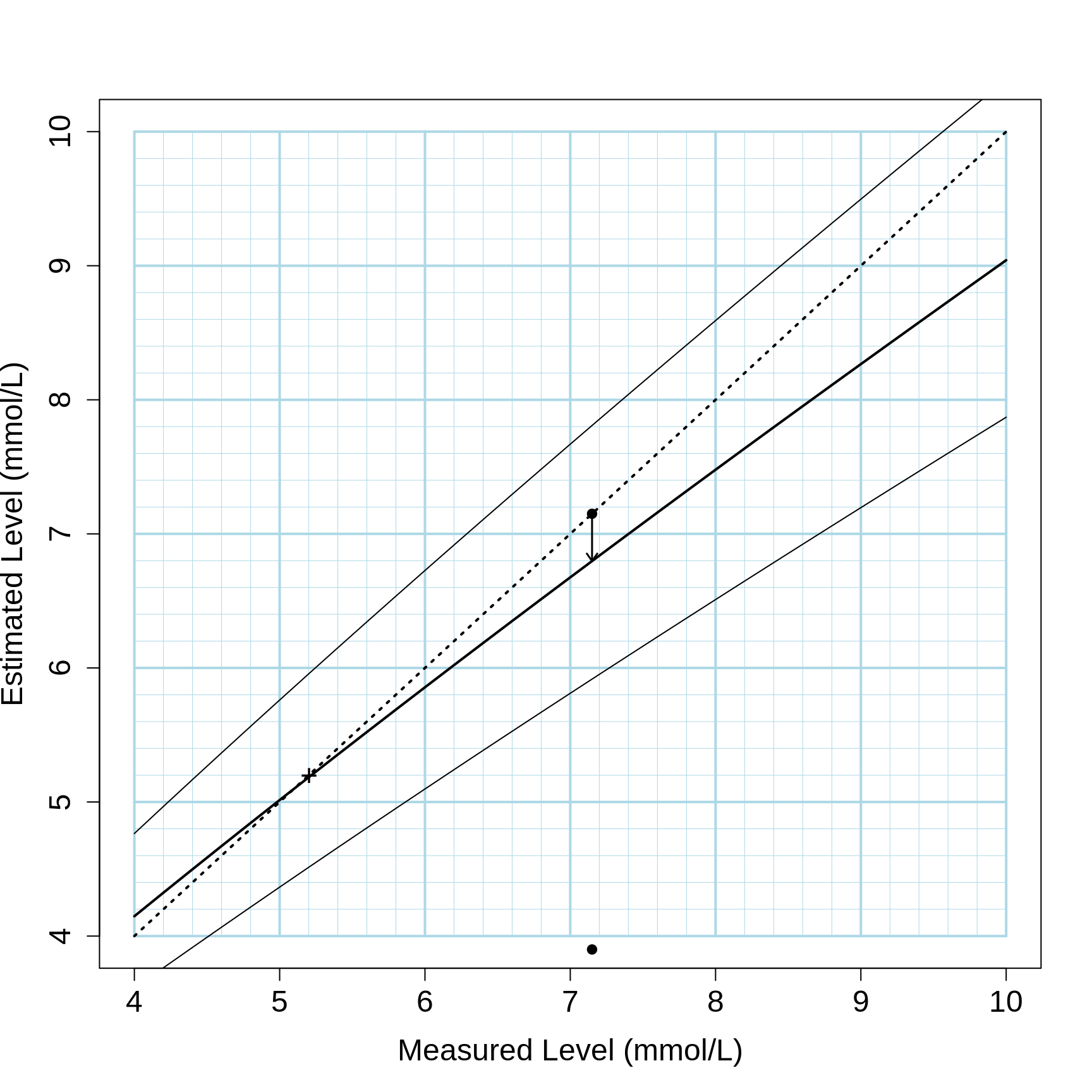
Figure 3.12: A Person's estimated true cholesterol level from one measurement for a population of individuals where the mean is 5.2 mmol/L (i.e, at the time of the article, men less than 35 and women less than 45 years old). The thicker solid line indicates the estimated true level, the thinner solid lines are 80% confidence intervals. The dotted diagonal line is an equivalence line. The arrow shows the amount by which a single measurement of 7.15 mmol/L is shrunk towards the population mean, to a rcorrected value of 6.8 mmol/L.

Below, we show the detailed calculations for a person with a single measurement of 7.15 mmol/L. For now, just focus on the items shown in red (the prior distribution for \(\theta\), blue (the 7.15 for the individual, and the associated likelihood function) and green (the posterior distribution of \(\theta\)). All the calculations are on the log scale.

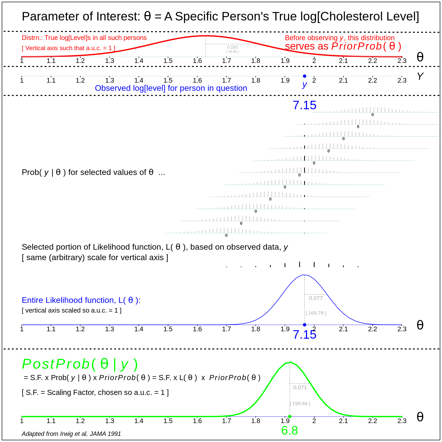
Figure 3.13: Worked example, for a person with a measured value of 7.15

combine estimates of different precisions into one more precise estimate, and do so using the same mathematical laws that are used in the Bayesian approach!]

Example 4

We end with a strking example of the limitations of using one-at-a-time frequentist intervals, each in isolation from the next. It is based on the example in this classic article.

The task is to predict each player's batting average over the remainder of the season using only the data from the first 4 weeks of the season. Since it proved difficult to replicate their selection croteria, we used instead the first 40 of these players.

The numbers of at bats per player up to mid April ranged from 44 to 73 (median 60 ). Efron and Morris used a constant 45. The numbers from mid April to the end of September ranged from 511 to 611 (median 542 ), or about 9 times as many as in the initial sample.

Clearly, the extreme results in these first 4 weeks were poor estimates of the perfornmances during the rest of the season. They 'shrunk' quite a bit.

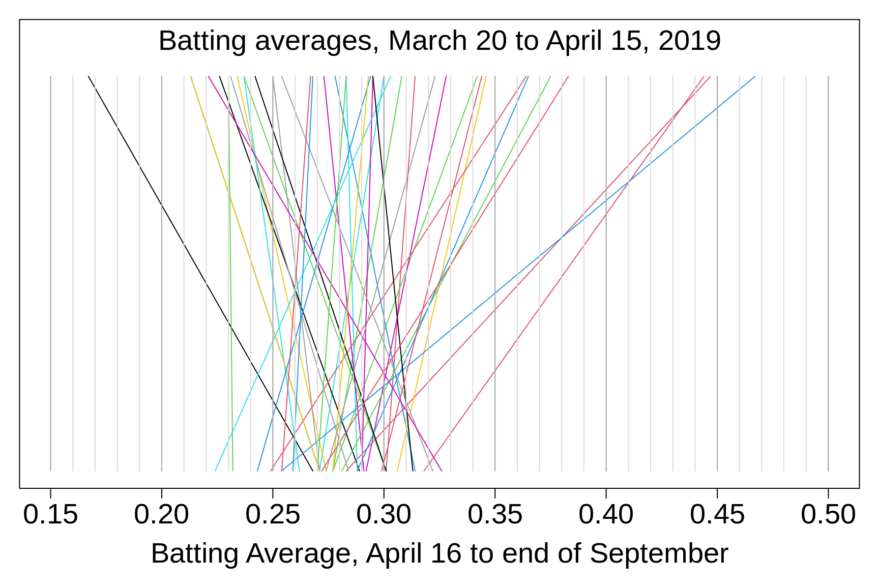
Figure 3.14: Batting averages of selected Major League baseball players, 2019

Across the performances up to mid April, the variance is a lot more than the variances in their 'real' (longer-term, remaining) performances. Thus, only about portion of it reflects the variance of the player-specific true (long-term) success rates. Will will quantify these later, below.

The individual binomial-based point estimates and frequentist confidence intervals we could construct (see next section) do not use the knowledge that individual season-long averages are confined to a narror band between say 0.225 and 0.325. Thus, many of them will not come close to or 'trap' the eventual individual longer-term batting averages. The correct way to make better frequentist intervals is to consider the family of players as an ensemble. If we label an randomly selected player as 'rs' say, then the long-run average \(\pi_{rs}\) is thought of (modelled) as drawn from the distribution (family) of long-run averages. A slightly simplified (for display and didactic purposes) version of this is shown in this figure.

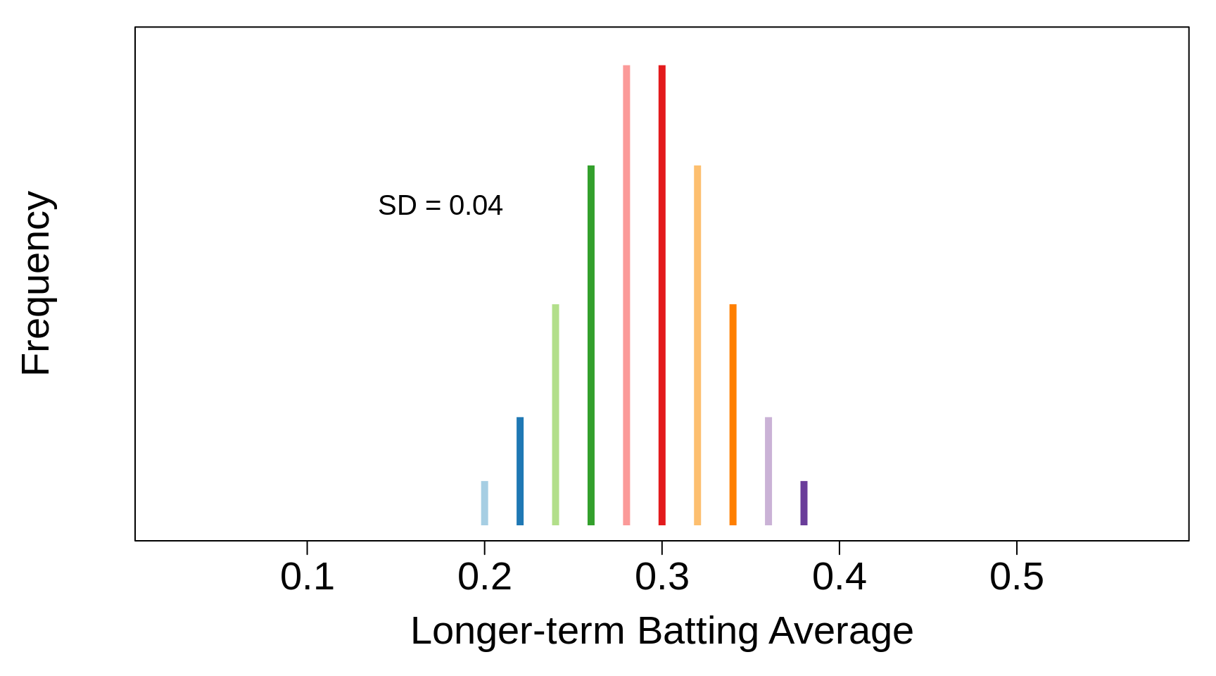
Figure 3.15: Simplified Distribution, for learning purposes, of Long-term Batting averages of Major League baseball players. Mean = 0.290; SD = 0.040.

How then should we think of (model) rs's short-term average? To make it concrete, suppose the number of at bats was \(n_{rs}\) = 60, and that we observed 21/60 hits. A natural way is to view the 21/60 as the end-result of (of having come to us in) two stages, each involving a random draw (i) \(\pi_{rs}\) was randomly drawn from the above distribution and then (ii) the number of hits was drawn from a binomial(\(n\)=60) distribution with the probability/proportion parameter \(\pi_{rs}\). Symbolically, we would describe the provenance of the \(y\) (= 21 for example) as \[(i) \ \pi_{rs} \sim distribution \ in \ previous \ figure ; \ \ (ii) \ \ y | \pi_{rs} \sim Binomial(n=60, \pi = \pi_{rs}).\]

provenance : The fact of coming from some particular source or quarter; origin, derivation. The history of the ownership of a work of art or an antique, used as a guide to authenticity or quality; a documented record of this. A distinction is sometimes drawn between the ‘origin’ and the ‘provenance’ of an article, as in 'A Canterbury origin is probable, Canterbury provenance is certain.' Forestry. The geographic source of tree seed; the place of origin of a tree. Also: seed from a specific location. Oxford English Dictionary

The bottom part of this next figure shows the frequencies of the possible end-results (possible observed short term averages). The colours show their 'provenance'. The top part shows the provenance of the '21/60' short-term averages in particular. Note the direction of the arrow, showing the reverse-engineering, from what we observe (the 21/60) back to where (who) it could have arisen from. The use of reverse probabilities is at the heart of the Bayesian approach. In his worked example, when Bayes wrote about 'the exact probability of all conclusions based on induction', his conclusions referred to the origin (original location, unknown) of a billiard ball, and his data referred to the locations where it came to rest in a number of trials.

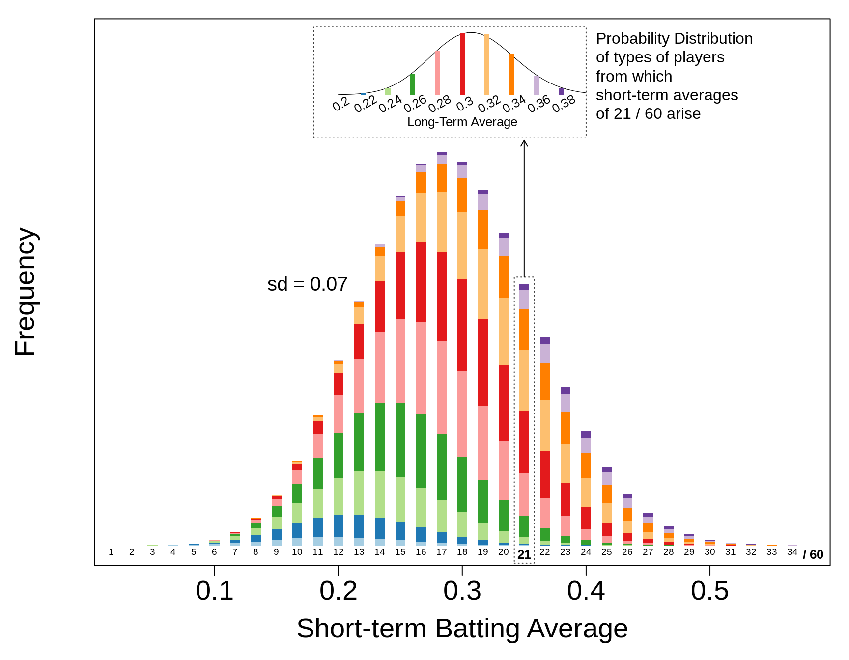
Figure 3.16: The bottom frequency distribution shows the expected frequencies of Short-term Batting averages from n = 60 at bats by types of players shown in previous figure. For each possible short-term average, the colours of their components show their 'provenance', i.e., which types of player this average arises from, and the relative contributions from each type. As an example, highlighted, within the column enclosed by a dashed line, is the provenance of the short-term averages that equal 21/60 = 0.350. In a real application, after n=60, IF ALL ONE KNEW WAS THE 21/60, one would not know which type of player, i.e., which colour, one was observing. Nevertheless, the theoretical calculations show that a short-term average of 21/60 = 0.350 is more likely to have been produced by a player who bats 0.320 or 0.300 or even lower, that one who bats 0.350 or or 0.360 or higher. Much more of the probability distribution lies to the left of the 0.350 than to the right of it! So we need to 'shrink' the observed 0.350 towards the 0.290.

Efron and Morris give a specific formula for merging the initial information (the 'centre' of 0.290) with the new information (the 21/60 = 0.350). the 'shrunken' estimate of the long-term average is a compromise, a weighted average, with the weights determined by the precision of the 21/60 (determined mainly by the 60) and the narrowness of the 'parent' distribution. We don't need to get into these at this stage.

But, we will address a question some of you may already have concerning the batting average example, compared with the cholesterol example. In the cholesterol example, the 'prior' (or population) distribution of individuals' true levels would be reasonably well known already. But in the baseball example, even though they had easy access to all of players' previous years of data, Efron and Morris did not use any historical data. Instead, they use a 'contemporaneous' prior: they inferred what the location and spread of the distribution shown in the second of our three baseball figures, just from the March to Aril 15, 2019 numbers shown along the top of the first figure. They did this by subtraction. In the simplest case, if all the short-term averages were based on the same number (\(n\)) of at bats (Efron and Morris used \(n\) = 45), we have the following variance (V) formula
\[V[short.term.averages] = V[long.term.averages] + \ V[binomial.proportion \ based \ on \ n.]\] They got to measure the left hand quantity empirically from their data on April 26 / May 3, 1970, and they knew from mathematical statistics that the rightmost quantity is of the order of \(0.3 \times 0.7 \ / \ 45\) = 0.0047. Thus they could deduce the spread of the long-term averages.

In our 2019 data, the numbers of early-season at bats vary from player to player, but we will simplify the math by taking a typical \(n\). Across the performances up to mid April, the (rounded) variance of the individual batting averages, (i.e., the left-hand \(V\) in the above equation) is 0.004640. The binomial variation that you would see with \(n\)'s of the order of 60 is approximately 0.003570. Player-specific true proportions vary from maybe 0.225 to 0.325. [for example, at \(\pi\) =0.30 and \(n\) = 60, the binomial variance is 0.30 * 0.70 / 60 = 0.003500.] Thus, by solving the equation \[0.004640 = V[long.term.averages] + \ 0.003500\]

we can back-calculate that the variance of the player-specific true (long-term) success rates is only about 0.001070. [The square root of this, sd = 0.033, broadly fits with the spead we see in the performances during the remainder of the season: the averages range from 0.224 to 0.326.]

To distinguish it from the typical Bayes approach, this double use of the data is sometime referred to as an 'Empirical Bayes' approach.

Empirical Bayes methods are procedures for statistical inference in which the prior distribution is estimated from the data. This approach stands in contrast to standard Bayesian methods, for which the prior distribution is fixed before any data are observed. Despite this difference in perspective, empirical Bayes may be viewed as an approximation to a fully Bayesian treatment of a hierarchical model wherein the parameters at the highest level of the hierarchy are set to their most likely values, instead of being integrated out. Empirical Bayes, also known as maximum marginal likelihood, represents one approach for setting hyperparameters. Wikipedia, 2020.04.15

3.1.4 The Bayesian Bottom Line

• As the examples all show, the Bayesian approach allows for direct-speak about parameters, without any of the 'legalese' we will have to use when using the frequentist approach.

• Because the end-product is a probability distribution for the parameter (\(\theta\) say), we can directly talk about the (pre-) and post-data probability that, say,
• \(\theta > 0,\) or (for any prespecified values \(A\) and \(B\))
• \(A < \theta < B\), or
• \(\theta > A\) or
• \(\theta < B\), or, as in the case of hemophilia carriage,

• \(\theta = Yes\) or \(\theta = No.\)

• If \(\theta\) = batting average for the remainder of season,

• Prob(a 21/60 player will have \(\theta \ge\) .350) = 0.11 [see Fig]

• Likewise, if we fix a desired probability \(P\), we can calculate \(\theta\) values \(\theta_{lower}\) and \(\theta_{upper}\) such that
• Prob( \(\theta > \theta_{lower}) = P\), or
• Prob( \(\theta < \theta_{upper}) = P\), or

• Prob( \(\theta_{lower} < \theta < \theta_{upper}) = P\).

• Again, if \(\theta\) = batting average for the remainder of season, then, in the case of a 21/60 player,

• Prob(0.245 < \(\theta\) < 0.377) = 0.95.

• Contrast this with the 95% frequentist confidence interval, based only on the 21/60, and not on the knowledge that (historically, or even by back-calculation just from the early 2019 data) most players' batting averages for a year are between 0.225 and 0.325,

• \(\theta_{lower}\) = 0.231 ; \(\theta_{upper}\) = 0.484) = 0.95.

Can this shrinkage be done without 'priors'?

3.2 Frequentist approach

In contrast to the seamless and unified Bayesian approach, the Frequentist approach is more fragmented, and is typically taught in two parts: tests of null hypotheses concerning a parameter or process, and confidence intervals (CI's).

Whereas we -- like others -- wish to downplay tests and elevate CI's, it is easier to start with tests. Don't take this to mean they are more scientifically relevant -- in most applications they are not. But it is difficult to learn the principle behind frequentist CIs without knowing what tests of null hypotheses are.

In their chapter 11, Null hypotheses and p-values, Clayton and Hills tell us

With most probability models there is one particular value of the parameter which corresponds to there being no effect. This value is called the null value, or null hypothesis. For a parameter \(\theta\) we will denote this null value by \(\theta_0\). In classical statistical theory, considerable emphasis is placed on the need to disprove (or reject) the null hypothesis before claiming positive findings, and the procedures which are used to this end are called statistical significance tests. However, the emphasis in this theory on accepting or rejecting null hypotheses has led to widespread misunderstanding and misreporting in the medical research literature. In epidemiology, which is not an experimental science, the usefulness of the idea has been particularly questioned. Undoubtedly the idea of statistical significance testing has been overused, at the expense of the more useful procedures for estimation of parameters which we have discussed in previous chapters. However, it remains useful. A null hypotheses is a simplifying hypothesis and measuring the extent to which the data are in conflict with it remains a valuable part of scientific reasoning. In recent years there has been a trend away from a making a straight choice between accepting or rejecting the null hypothesis. Instead, the degree of support for the null hypothesis is measured, for example using the log likelihood ratio at the null value of the parameter. Clayton and Hills, p96. [Their illustration involved an investigation of the possible linkage of the HLA locus to nasopharyngeal cancer susceptibility]

In Chapter 2.4, Classical hypothesis testing, Gelman and Hill tell us

The possible outcomes of a hypothesis test are 'reject' or 'not reject.' It is never possible to 'accept' a statistical hypothesis, only to find that the data are not sufficient to reject it.
.
Comparisons of parameters to fixed values and each other: interpreting confidence intervals as hypothesis tests
.
The hypothesis that a parameter equals zero (or any other fixed value) is directly tested by fitting the model that includes the parameter in question and examining its 95% interval. If the interval excludes zero (or the specified fixed value), then the hypothesis is rejected at the 5% level.
Testing whether two parameters are equal is equivalent to testing whether their difference equals zero. We do this by including both parameters in the model and then examining the 95% interval for their difference. As with inference for a single parameter, the confidence interval is commonly of more interest than the hypothesis test. For example, if support for the death penalty has decreased by 6% \(\pm\) 2.1%, then the magnitude of this estimated difference is probably as important as that the change is statistically significantly different from zero. The hypothesis of whether a parameter is positive is directly assessed via its confidence interval. If both ends of the 95% confidence interval exceed zero, then we are at least 95% sure (under the assumptions of the model) that the parameter is positive. Testing whether one parameter is greater than the other is equivalent to examining the confidence interval for their difference and testing for whether it is entirely positive.

In section 2.5, Problems with statistical significance, they warn that

A common statistical error is to summarize comparisons by statistical significance and to draw a sharp distinction between significant and nonsignificant results. The approach of summarizing by statistical significance has two pitfalls, one that is obvious and one that is less well known. First, statistical significance does not equal practical significance. For example, if the estimated predictive effect of height on earnings were $10 per inch with a standard error of $2, this would be statistically but not practically significant. Conversely, an estimate of $10,000 per inch with a standard error of $10,000 would not be statistically significant, but it has the possibility of being practically significant (and also the possibility of being zero; that is what “not statistically significant” means).
.
The second problem is that changes in statistical significance are not themselves significant. By this, we are not merely making the commonplace observation that any particular threshold is arbitrary — for example, only a small change is required to move an estimate from a 5.1% significance level to 4.9%, thus moving it into statistical significance. Rather, we are pointing out that even large changes in significance levels can correspond to small, nonsignificant changes in the underlying variables.

They illustrate the application of basic statistical methods with a story, in which, a couple of years before, they received a fax, entitled HELP!, from a member of a residential organization:

Last week we had an election for the Board of Directors. Many residents believe, as I do, that the election was rigged and what was supposed to be votes being cast by 5,553 of the 15,372 voting households is instead a fixed vote with fixed percentages being assigned to each and every candidate making it impossible to participate in an honest election.

Gelman and Hill devote 3 pages to their analysis, which led them to

conclude that the intermediate vote tallies are consistent with [the null hypothesis of] random voting. As we explained to the writer of the fax, opinion polls of 1000 people are typically accurate to within 2%, and so, if voters really are arriving at random, it makes sense that batches of 1000 votes are highly stable. This does not rule out the possibility of fraud, but it shows that this aspect of the voting is consistent with the null hypothesis.

Cox acknowledges

a large and ever-increasing literature on the use and misuse of significance tests. This centres on such points as:

1. Often the null hypothesis is almost certainly false, inviting the question why is it worth testing it?
   
2. Estimation of \(\theta\) is usually more enlightening than testing hypotheses about \(\theta\).
   
3. Failure to ‘reject’ \(H_0\) does not mean that we necessarily consider \(H_0\) to be exactly or even nearly true.
   
4. If tests show that data are consistent with \(H_0\) and inconsistent with the minimal departures from \(H_0\) considered as of subject-matter importance, then this may be taken as positive support for \(H_0\) , i.e., as more than mere consistency with \(H_0\).
   
5. With large amounts of data small departures from \(H_0\) of no subject-matter importance may be highly significant.
   
6. When there are several or many somewhat similar sets of data from different sources bearing on the same issue, separate significance tests for each data source on its own are usually best avoided. They address individual questions in isolation and this is often inappropriate.
   
7. The p-value is not the probability that \(H_0\) is true.

He continues

Discussion of these points would take us too far afield. Point 7 addresses a clear misconception. The other points are largely concerned with how in applications such tests are most fruitfully applied and with the close connection between tests and interval estimation. The latter theme is emphasized below. The essential point is that significance tests in the first place address the question of whether the data are reasonably consistent with a null hypothesis in the respect tested. This is in many contexts an interesting but limited question. The much fuller specification needed to develop confidence limits by this route leads to much more informative summaries of what the data plus model assumptions imply.

Using some classic examples as illustrations, we now begin now with our own home-grown explanations

3.2.1 (Frequentist) Test of a Null Hypothesis

Use: To assess the evidence provided by sample data in favour of a pre-specified claim or 'hypothesis' concerning some parameter(s) or data-generating process. As do confidence intervals, tests of significance make use of the concept of a sampling distribution.

Example 1

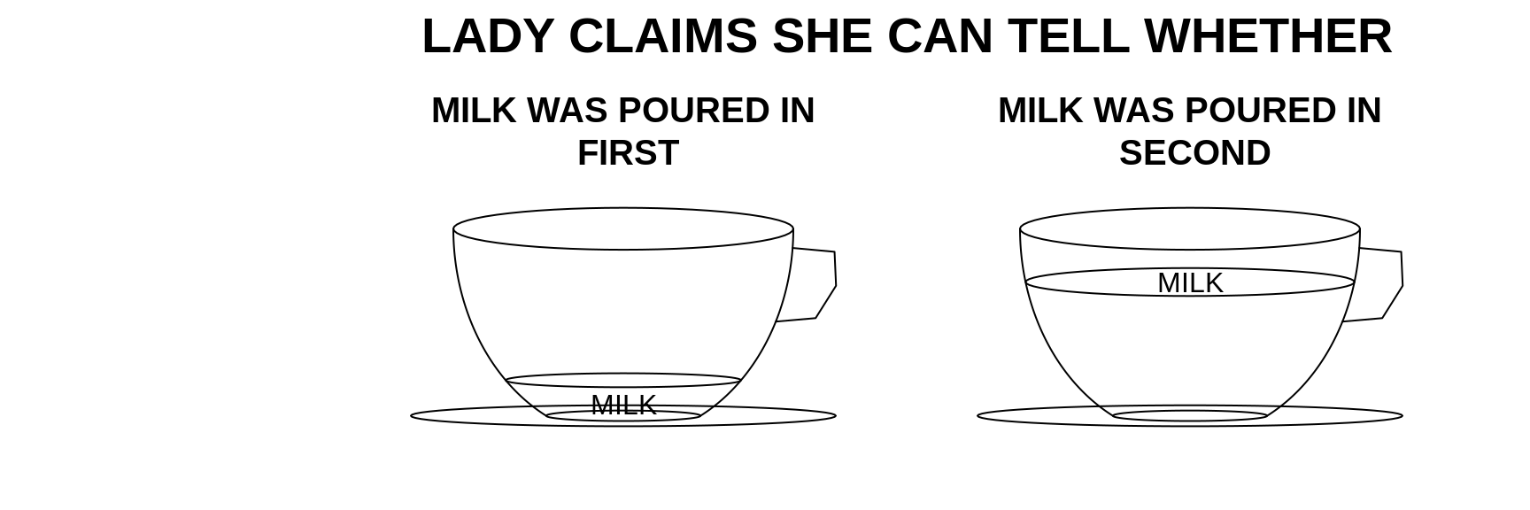
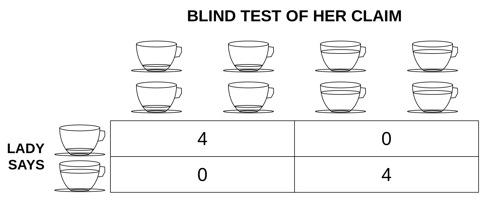
The Mathematics of a Lady Tasting Tea. Whether the sensory experiment was actually carried out has been the subject of subsequent articles. In 2002, the phrase 'Lady Tasting Tea':' was used as the title, and How Statistics Revolutionized Science in the Twentieth Century the subtitle of this book which you can borrow from the McGill Librray. Here is a link to an online copy of Fisher's 1935 book Design of Experiments

Fisher continued

It is usual and convenient for experimenters to take 5 per cent. as a standard level of significance, in the sense that they are prepared to ignore all results which fail to reach this standard, and, by this means, to eliminate from further discussion the greater part of the fluctuations which chance causes have introduced into their experimental results. No such selection can eliminate the whole of the possible effects of chance coincidence, and if we accept this convenient convention, and agree that an event which would occur by chance only once in 70 trials is decidedly "significant," in the statistical sense, we thereby admit that no isolated experiment, however significant in itself, can suffice for the experimental demonstration of any natural phenomenon; for the one chance in a million" will undoubtedly occur, with no less and no more than its appropriate frequency, however surprised we may be that it should occur to us. In order to assert that a natural phenomenon is experimentally demonstrable we need, not an isolated record, but a reliable method of procedure. In relation to the test of significance, we may say that a phenomenon is experimentally demonstrable when we know how to conduct an experiment which will rarely fail to give us a statistically significant result.

In this example, the result was the most extreme that it could be. But, Fisher asked, 'what should be our conclusion if, for each kind of cup, her judgments are 3 right and 1 wrong?

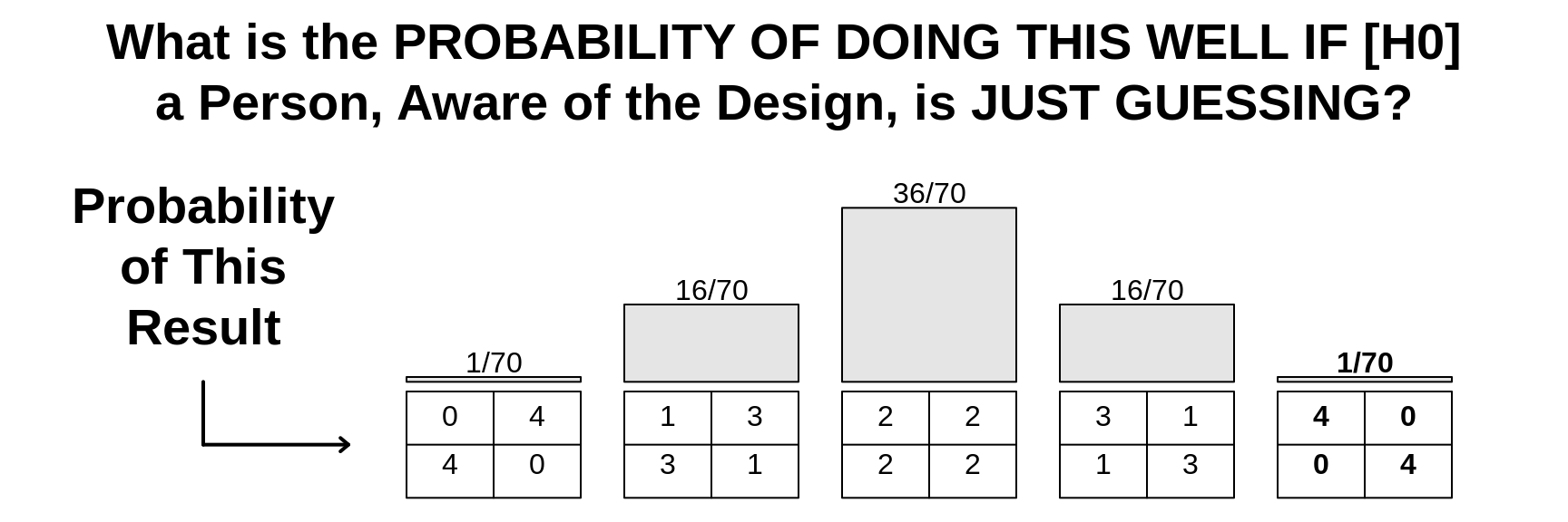
It is obvious, too, that 3 successes to 1 failure, although showing a bias, or deviation, in the right direction, could not be judged as statistically significant evidence of a real sensory discrimination. For its frequency of chance occurrence is 16 in 70, or more than 20 per cent. Moreover, it is not the best possible result, and in judging of its significance we must take account not only of its own frequency, but also of the frequency for any better result. In the present instance "3 right and 1 wrong" occurs 16 times, and "4 right" occurs once in 70 trials, making 17 cases out of 70 as good as or better than that observed. The reason for including cases better than that observed becomes obvious on considering what our conclusions would have been had the case of 3 right and 1 wrong only 1 chance, and the case of 4 right 16 chances of occurrence out of 70. The rare case of 3 right and 1 wrong could not he judged significant merely because it was rare, seeing that a higher degree of success would frequently have been scored by mere chance.

JH would add: if the experiment involved 200 cups of each kind, and she only got 106 right? The probability of exactly this number is just 4% whereas the probability of at least this number is 14%

Example 2

Preston-Jones vs. Preston-Jones (1946-1951), excerpted from here.

The facts were as follows: The husband (the appellant) was married to the wife (the respondent) on April 14, 1941, at Brymbo in the county of Denbigh. Jean, a child of the marriage, was born on April 15, 1942. On August 13, 1946, a second child was born to the wife. The husband, alleging that this child was not his child and founding on the circumstances of his birth a charge of adultery against the wife, on November 8, 1946, presented a petition to the High Court for the dissolution of his marriage. He alleged that the said child was conceived some time between August 29, 1945, and February 13, 1946, during the whole of which period of time [he] was absent from the United Kingdom and . . . the [wife] was resident in the United Kingdom and that the child must therefore have been conceived as the result of an act of adultery.

The petition was first heard by His Honour Commissioner Burgis, who dismissed it. The husband appealed to the Court of Appeal and that court allowed the appeal, [...] set aside the order of the commissioner and directed the petition to be reheard before another judge.

The petition was reheard on March 24, 1949, by Mr. Commissioner Blanco White, K.C. He concluded:

I am not satisfied beyond a reasonable doubt that adultery has been committed. ... The question reduces itself to the simple question as to whether the court's judicial knowledge of natural laws enables it to say without any satisfactory evidence that 360 days between coition and birth is an impossible period and whether, if that period elapsed, a woman, who is, so far as the rest of the evidence goes, a respectable woman, is to be convicted of adultery. I think not.

He dismissed the petition.

The husband appealed to the Court of Appeal, which on July 22, 1949, set aside the commissioner's order and ordered the cause to be reheard by a judge of the High Court if possible. The husband appealed to the House of Lords, asking that a decree for dissolution of the marriage should be made. The wife cross-appealed, asking that the petition should be dismissed.

The final paragraph of the lengthy of opinions of the five Lords at the end of 1950:

your text My Lords, I do not think it open to doubt that a time must come when, with the period far in excess of the normal, the court may properly regard its length as proving the wife's adultery beyond reasonable doubt, and decree accordingly. But, as has so often been pointed out, the difficulty is to know where to draw the line. The reported cases naturally tend to creep up on each other and there is little sound guidance to be gleaned from authority. If a line has to be drawn I think it should be drawn so as to allow an ample and generous margin, for it may be as difficult for the wife to prove a freak of nature as for anyone else; and it need hardly be added that, before acting on the length of the period, due regard must be paid to any other relevant evidence. But I do not find it possible to go further and lay down any hard and fast rule capable of general application. In my opinion there is nothing in the testimony here, or in the facts of which judicial notice may be taken, to justify fixing a specific period and holding that, in the absence of evidence to the contrary, anything more would, but anything less would not, prove adultery beyond reasonable doubt. If, in the light of a full and exhaustive inquiry, the line could be thus fixed it might well be that the period of 360 days would come near or even cross it. But, however that may be, I am not prepared to decide this case merely on the fact that a period of that duration has been established. I prefer to relate my conclusion to the evidence as a whole and, for the reasons already given, I think it should have satisfied the learned commissioner beyond reasonable doubt. I would therefore allow the appeal and dismiss the cross- appeal.

Appeal allowed.

The following is from this 'bible' for those who became parents in the 1970s

What Are the Chances of Delivering on Time?

In over 17,000 cases of pregnancy carried beyond the twenty seventh week, 54 per cent delivered before 280 days, 4 percent had their babies either the week before or the week after the calculated date, and 74 per cent within a two-week period before or after the anticipated day of birth.
On the basis of these data one can calculate the likelihood which the average woman faces when carrying a single infant, not twins, of having her baby, during each week after the twenty-seventh week from the first day of her last menstrual period.

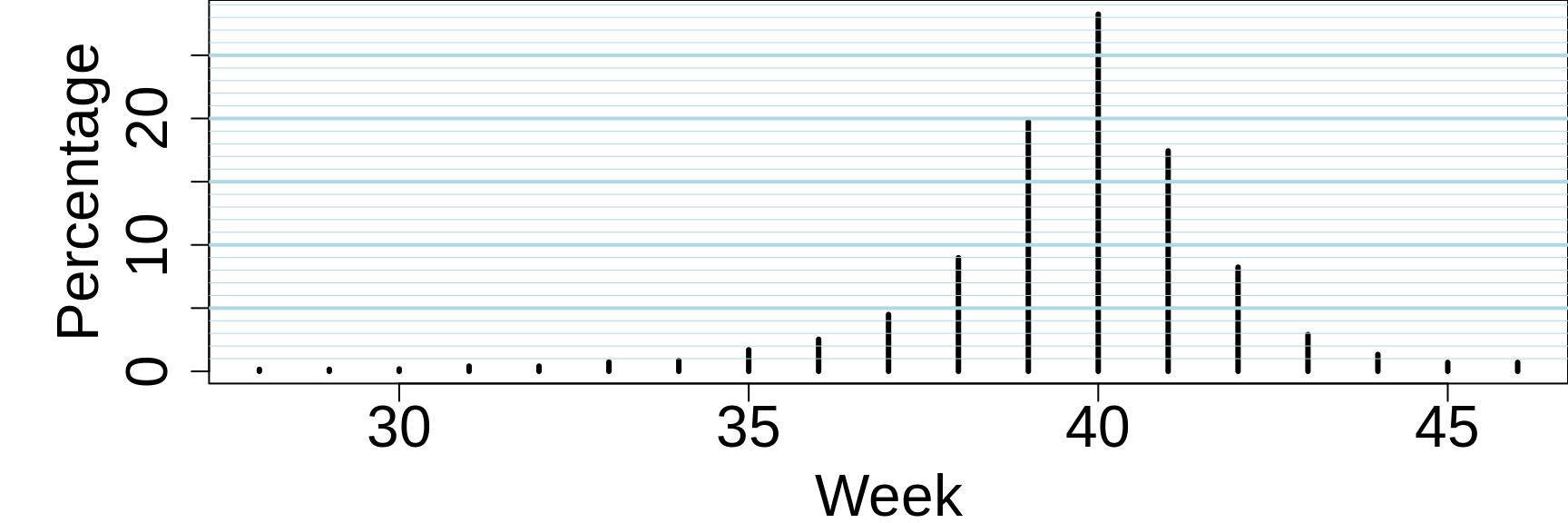
The author then presents a frequency distribution in 19 rows and 3 columns, with the headers Weeks (27, 28, ... 45, 46+), Days (189-196, 196-203, ... 308-315, 315+) and Approximate Chance (1:625, 1:625, 1:525, ... 1:140, 1:140). We have converted it to a graphic.

The author does on to say that

Another reliable study has shown that 40 per cent of women go into labor within a ten-day period — five days before and five days after the calculated date, and nearly two thirds within plus or minus ten days of the expected time.

Altman, writing in the BMJ in 1980, gives a graph based on 1970 data from England.

In that (pre-ultrasound) era, some of the variation was dues to dating errors. But a 2013 article, based on carefully collected daily urine samples found that even with the precise measuremet of the timing of pregranct that these samples provides the length of human pregnancies can vary naturally by as much as five weeks

Normally, women are given a date for the likely delivery of their baby that is calculated as 280 days after the onset of their last menstrual period. Yet only four percent of women deliver at 280 days and only 70% deliver within 10 days of their estimated due date, even when the date is calculated with the help of ultrasound.
Now, for the first time, researchers in the USA have been able to pinpoint the precise point at which a woman ovulates and a fertilised embryo implants in the womb during a naturally conceived pregnancy, and follow the pregnancy through to delivery. Using this information, they have been able to calculate the length of 125 pregnancies.
"We found that the average time from ovulation to birth was 268 days -- 38 weeks and two days," said Dr Anne Marie Jukic, a postdoctoral fellow in the Epidemiology Branch at the National Institute of Environmental Health Sciences (Durham, USA), part of the National Institutes for Health. "However, even after we had excluded six pre-term births, we found that the length of the pregnancies varied by as much as 37 days.
"We were a bit surprised by this finding. We know that length of gestation varies among women, but some part of that variation has always been attributed to errors in the assignment of gestational age. Our measure of length of gestation does not include these sources of error, and yet there is still five weeks of variability. It's fascinating."
The possibility that the length of pregnancies can vary naturally has been little researched, as it is impossible to tell the difference between errors in calculations and natural variability without being able to measure correctly the gestational age of a developing fetus. Previous studies conducted as long ago as the 1970s and 1980s had used the slight rise in a woman's body temperature at waking as a way of detecting when ovulation occurred. This is an inexact measurement and cannot be used to detect when the embryo actually implants in the womb. Science Daily.

But even if the variation is still (naturally) large, the original (1849) ruling in the Preston-Jones case seems extreme. Altman asks us to look at the distribution of length of gestation in his Fig 1, 'which the judges apparently did not do.' Altman himself thought that

most people would feel that the husband was hard done by. Even If this case were heard now, where would you draw the line on the basis of (Altman's) fig 1 ?
This case illustrates a failure to use statistical methods when they ought to have been used, a fairly common occurrence. Saying that an event is possible is quite different from saying that it has a probability of, say, one in 100,000. Although not an example from medical research, this case concerne essentially the same difficulty as in many more frequentl encountered problems, such as denning hypertension or obesity Everything varies; it is in trying to draw lines between good and bad, high and low, likely and unlikely, and so on, that many problems arise. Although statistics cannot answer a given question, they can often shed considerable light on the problem. Altman, 1980.

Today, JH would add that we should also consider, as those who heard the case did, the other evidence and testimony presented in the case. (We will come back to this when discussing the prosecutor's fallacy.)

3.2.2 Ingredients and methods of procedure in a statistical test

The bullet point following each item is specific to the Preston-Jones case.

1. A claim about a parameter (or about the shape of a distribution, or the way a lottery works, etc.). Note that the null and alternative hypotheses are usually stated using Greek letters, i.e. in terms of population parameters, and in advance of (and indeed without any regard for) sample data.

• Parameter (unknown): Date of Conception
  CLAIMS by husband (h) and by wife (w)
  H\(_0\)(w): Date of Conception < HUSBAND LEFT
  H\(_A\)(h): Date of Conception > HUSBAND LEFT

2. A probability model (in its simplest form, a set of assumptions) which allows one to predict how a relevant statistic from a sample of data might be expected to behave under H\(_0\).

• A probability model for statistic; examples: Gaussian, Empirical (common wisdom, and expert testimony at the time). In the 1949 hearing, the Commissioner referred to the 'court's judicial knowledge of natural laws

3. A probability level or threshold or dividing point below which (i.e. close to a probability of zero) one considers that an event with this low probability 'is unlikely' or 'is not supposed to happen' or 'just doesn't happen'. This pre-established limit of extreme-ness is referred to as the \(\alpha\) level of the test.

• Fisher, in his treatment of the tea-tasting experiment, allowed that 'It is open to the experimenter to be more or less exacting in respect of the smallness of the probability he would require before he would be willing to admit that his observations have demonstrated a positive result.' Hovever, he is in part responsible for the 0.05 probability threshold commonly used today.

• None of those who pronounced on the Preston-Jones case gave a value for this.

Denning, L.J., 'thought that, according to the ordinary knowledge of mankind, a 360-day normal baby is impossible; and the courts should not assert that it is possible unless there is direct medical evidence to that effect.'

4. A sample of data, which under H\(_0\) is expected to follow the probability laws in (2)

• \(y\) = 360 days between when husband left and baby was born [the House of Lords account mentions 3 different departure dates, August 13, 17, and 29, but the Lords all spoke of 360 days in their deliberations]

5. The most relevant statistic (e.g. \(\bar{y}\) if interested in inference about the parameter \(\mu\))

• 360 - 280 = 80 days (here \(n\) = 1, so \(y\) and \(bar{y}\) are the same)

6. The probability of observing a value of the statistic as extreme or more extreme (relative to that hypothesized under H\(_0\)) than we observed. This is used to judge whether the value obtained is either 'close to' i.e. 'compatible with' or 'far away from' i.e. 'incompatible with', H\(_0\). The 'distance from what is expected under H0' is usually measured as a tail area or probability and is referred to as the 'P-value' of the statistic in relation to H\(_0\).

• P = Prob[ 360 or 361 ... | \(\mu\) = 280]. Although it was not quantified, it was taken to be quite small.

• IN PASSING: This example re-inforces Fisher's explanation as to why it is the tail area (the probablities of outcomes AS extreme OR MORE extreme than the observed one that is relevant, not the probability of the observed one. Even though day 280 is close to the mode of the distribution, fewer than 5% of babies are born on day 280, and only about 4% on day 285. This 'just 4%' does not make being '5 days late' suspicious: more than 25% of babies are born this late or later.

7. A comparison of this 'extreme-ness' or 'unusualness' or 'amount of evidence against H\(_0\)' or P-value with the agreed-on 'threshold of extreme-ness'. If it is beyond the limit, H\(_0\) is said to be 'rejected'. If it is not-too-small, H0 is 'not rejected'. These two possible decisions about the claim are reported as 'the null hypothesis is rejected at the P = \(\alpha\) significance level' or 'the null hypothesis is not rejected at a significance level of 5%'.

• Mr. Commissioner Blanco White, K.C., who heard the petition in 1949, didn't tell us his threshold, but his use of the word 'impossible' suggests it might have been zero.
  Bucknill, L.J. of the Court of Appeal noted that the commissioner in his judgment said it appeared to be a pure question of law whether 360 days is an impossible period without any satisfactory scientific evidence to that effect.' Bucknill saw the case 'not in that light but rather as one where the court must balance the probabilities one against the other. On the one hand there is the very great improbability, I will not put it any higher, that a woman can, 360 days after coitus, give birth to a normal full-time child of 8 and a quarter pounds without any ifficult labour, and after a pregnancy which, according to the wife, was not unduly prolonged, but, on the contrary, was cut short. As against this high improbability there is the fact that the wife has put forward the case of a visit by the husband to her in November, a case which the commissioner has not accepted. If the matter rested there I should be in favour of allowing this appeal [siding wth the husband]. [if interested, see the origibal for why he ordered a re-hearing.] Denning, L.J., of the same Court of Appeal dissented, saying that 'the irresistible inference was that it was conceived in adultery. [...] according to the ordinary knowledge of mankind, a 360-day normal baby is impossible; and the courts should not assert that it is possible unless there is direct medical evidence to that effect.'
  In his summary, Lord Simonds said that since 'The result of a finding of adultery in such a case as this is in effect to bastardize the child', it 'is a matter in which from time out of mind strict proof has been required. But that does not mean that a degree of proof is demanded such as in a scientific inquiry would justify the conclusion that such and such an event is impossible. In this context at least no higher proof of a fact is demanded than that it is established beyond all reasonable doubt: see Head v. Head (18). To prove that a period of so many days between fruitful coition and the time of conception is in a scientific sense impossible is itself, I suppose, a scientific impossibility. The utmost that a court of law can demand is that it should be established beyond all reasonable doubt that a child conceived so many days after a particular coitus cannot be the result of that coitus.

Other Examples:

• Quality Control (it has given us the terminology)
• Taste-tests (see exercises )
• Jumping the gun in athletics
• After having had 3 NL sons, is potential-carrier mother a carrier?
• Adding water to milk..seeM&M2Example6.6p448
• Water divining..seeM&M2exercise6.44p471
• Randomness of U.S. Draft Lottery of 1970.. see M&M2 Example 6.6 p105-107, and 447-
• Births in New York City after the "Great Blackout"
• John Arbuthnot's "argument for divine providence"
• US Presidential elections: Taller vs. Shorter Candidate.
• Gelman and Hill, HELP. 50,000 votes
• Laplace average depth of the oceans is of the same order as the average height of the continents.
• Under the null hypothesis of the independence of the row and column factors, the expected value of the chi-square statistic calculated from a 2 \(\times\) 2 table is 4 - 1 = 3 (said Karl Pearson in 1900) or (2 - 1)\(\times\) (2 - 1) = 1 (said Ronald Fisher, and G Udny Yule in 1922).

The same arguments which explode the Notion of Luck may, on the other side, be useful in some Cases to establish a due comparison between Chance and Design. We may imagine Chance and Design to be as it were in Competition with each other for the production of some sorts of Events, and may calculate what Probability there is, that those Events should be rather owing to one than to the other... From this last Consideration we may learn in many Cases how to distinguish the Events which are the effect of Chance, from those which are produced by Design. Abraham de Moivre: 'Doctrine of Chances' (1719)

THE FIRST RECORDED P–VALUE??? by a physician no less!! "AN ARGUMENT FOR DIVINE PROVIDENCE, TAKEN FROM THE CONSTANT REGULARITY OBSERV'D IN THE BIRTHS OF BOTH SEXES." John Arbuthnot, 1667-1735 physician to Queen Anne Arbuthnot claimed to demonstrate that divine providence, not chance, governed the sex ratio at birth. To prove this point he represented a birth governed by chance as being like the throw of a two-sided die, and he presented data on the christenings in London for the 82-year period 1629-1710. Under Arbuthnot's hypothesis of chance, for any one year male births will exceed female births with a probability slightly less than one-half. (It would be less than one-half by just half the very small probability that the two numbers are exactly equal.) But even when taking it as one-half Arbuthnot found that a unit bet that male births would exceed female births for eighty-two years running to be worth only (1/2)82 units in expectation, or 1 4 8360 0000 0000 0000 0000 0000 a vanishingly small number. "From whence it follows, that it is Art, not Chance, that governs."

STIGLER : HISTORY OF STATISTICS

nificance levels can correspond to small, nonsignificant changes in the underlying variables. 2 separate issues Ho and intervals (treated together in Bayesian)

• Statistical Quality Control procedures [for Decisions] • Sample survey organizations: Confidence intervals • Statistical Tests of Hypotheses Unlike Bayesian inference, there is no quantified pre-test or pre- data "impression"; the ultimate statements are about data, conditional on an assumed null or other hypothesis. Thus, an explanation of a p-value must start with the conditional "IF the parameter is ... the probability that the data woul

3.3 Does the approach matter?

semantics