Chapter 4 Parameter Intervals

The objective of this first section is to provide simple examples of reverse engineering that show some of the logic behind statistical 'confidence intervals' for parameters. We begin with '100% confidence' intervals, and then, in section 2, we explain why we have to move to 'less-than-100% confidence' intervals, where things get a bit more nuanced. In both sections, we emphasize the reverse engineering, i.e, by using as our limits the worst-case or almost-worst-case scenarios involving the (unknown) values of the parameter that is being estimated.

4.1 '100% confidence' intervals

Example 1

Consider a very 'particularistic' parameter, the height of a particular building. There is nothing 'scientific' about the parameter, except maybe that we use tools of mathematical science (of trignometry) to measure it. Nevertheless, we will sometimes refer to it one of the generic symbols for a parameter, namely \(\theta.\)

Suppose you measure the height of this building by standing a known horizontal distance (e.g. 100 metres) from the bottom of the building and using an instrument to measure the angle between the horizontal and the top of the building. Suppose, as shown in the left panel of the Figure below, that the instrument gives a reading of 70 degrees.

Remembering from trigonometry that the tangent of a 70 degree angles is 2.75, the angle of 70 degrees suggests that the height of the building is \(\hat{\theta}\) = 275 metres. The 'hat' is statistical shorthand for 'estimate of.' Since it is sometimes referred to as a 'point estimate' of \(\theta\), we display the value using a dot or point.

After calculating this, you learn that the measuring instrument only displays the angle is to the nearest 10 degrees. This means that the true angle is somewhere between 65 and 75 degrees. [This is the same range you would get if it was dark and you used a laser pointer or flashlight attached to a wheel that rotates in fixed 10-degree steps, i.e., 5 degrees, 15 degrees, 25 degrees, etc. At 65 degrees, the light is visible on the building, but at 75 degrees, it goes above the building and shines into the sky.]

So you cannot say that the true height is exactly 275 metres. What can you say? And with what certainty?

You can put limits on the true height by asking what are the minimum and maximum heights that could have produced the observed reading of 70 degrees?

To do this you need to take the limits one at a time. The minimum angle that could have given the (rounded) readout of 70 degrees is 65 degrees, and this corresponds to a minimum height (lower limit) height of \(\theta_L\) = 214 metres. The maximum angle that could have given the readout of 70 degrees is 75 degrees, and this corresponds to a maximum height (upper limit) of \(\theta_U\) = 373 metres. Thus, assuming that the instrument is measuring the angle correctly, and then doing what you are told it does, you are 100% confident that the true height lies in the interval (214, 373). As is clear in the graph, this does not have the typical 275 \(\pm\) a single-number (or in sybols, \(\hat{\theta} \pm\) ME ['margin of error']) that we typically see in reports.

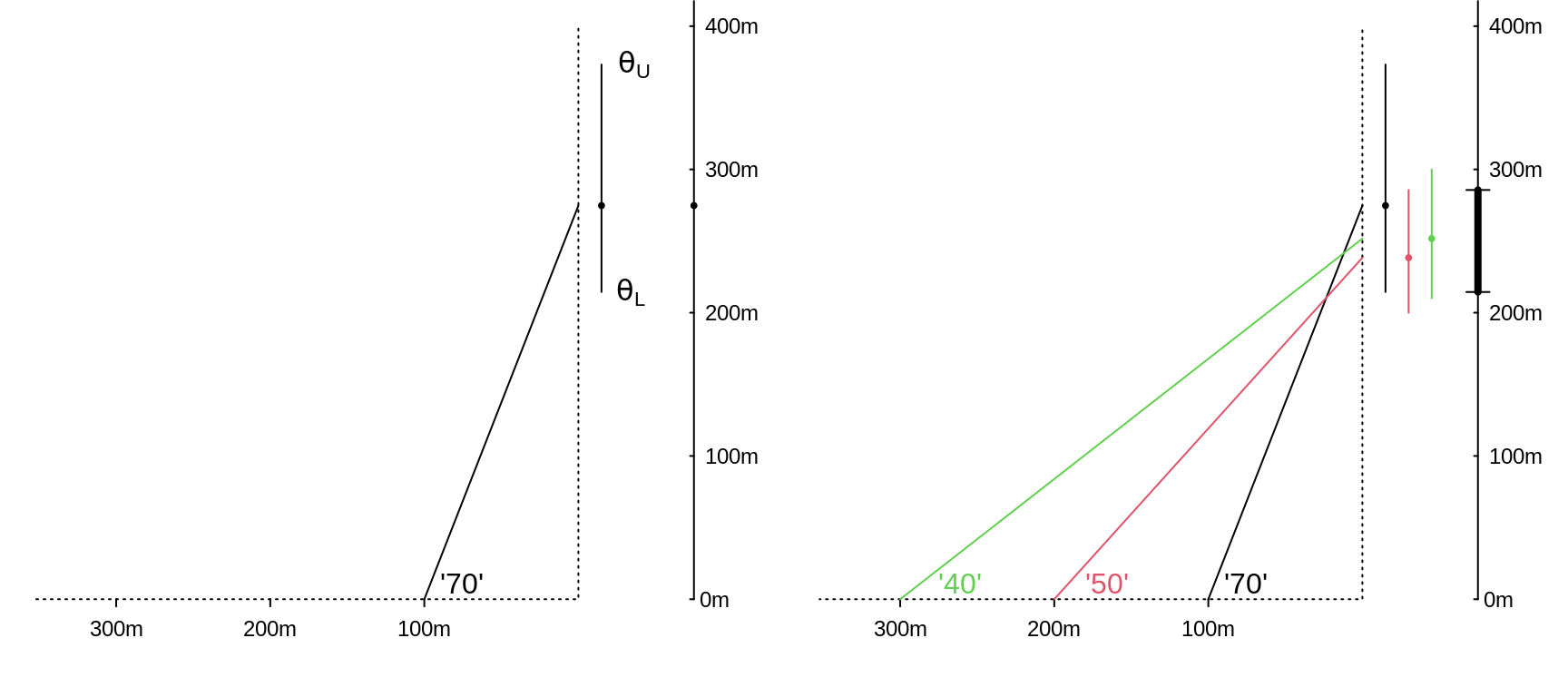
Figure 4.1: Estimating the height of an building by measuring subtended angles. The '70' in the left panel signifies that the real angle was somewhere between 65 and 75 degrees; thus the real height lies between the L and U limits of 214 and 373 metres. In the righ panel, the interval shown by the thicker black segment to the right of the 3 individual intervals is the set of parameter values common to all 3.

More data

The panel on the right shows how, by obtaining 3 measurements at 3 different distances, and finding the interval they have in common (the overlap), you can narrow the interval within which the true height must lie.

What allows us to be 100% confident in the parameter interval

The reason is the limited error range. How wide the error range is, and how many measurements one makes, determine how wide the parameter interval is.

Example 2

This one is less artificial, and indeed is motivated by a real court case in the late 1990s in Quebec, where a defendant's age (which would determine wheter he was tried in an adult or a juvenile court) was in doubt. He was adopted, while still a young child, from another country. Official birth records were not available, and his adoptive parents were able to get a cheaper airfare by claiming that he was under age 2 at the time. Bone age, and Tanner Staging, also known as Sexual Maturity Rating (SMR), an objective classification system used to track the development and sequence of secondary sex characteristics of children during puberty, were other pieces of information used by the judge.

For more on this topic of determining chronological age, see this article, entitled Many applications for medical statistics and thos one, entitled People smugglers, statistics and bone age, by UCL statistics professor and child growth expert, Tim Cole.

Again, the person's correct chronological age is a particularistic parameter, one that had nothing to do with science, or universal laws of Nature. But it can be estimated by using the laws of mathematics and statistics.

For didactic purposes, we will simplify matters, and assume that 'our' indirect method gives estimates such that if many of them were averaged, they would give the correct chronological age of the person (in statistical lingo, statisticians say that the method/estimator is 'unbiased'). However, as is seen below, the individual measurements vary quite a bit around the correct age. They can be off by as much as 25% (1/4th) in either direction. [In practice, a measuring instrument with this much measurement error would not be useful -- unless it was fast, safe, inexpensive, non-invasive, easily repetaed, and so on -- but we make the measurement variations this large just so we can see the patters more clearly on the graph!]. Another unrealistic feature of our 'measurement model' is that the 'error distribution' has a finite range. The shape of the error distribution doesn't come into the 100% 'confidence intervals' below, but it will matter a little bit -- but not a whole lot unless the sample size is small -- later on when we cut corners.

Consider first a single indirect measurement of chronological age, that yielded a value of 17.6 years.

Given what you know about the sizes of the possible errors, you cannot say that the true age is exactly 17.6 years What can you say? And with what certainty?

You can put limits on the true age by asking what are the minimum and maximum ages that could have produced the observed reading of 17.6 years.

To do this you need to consider the limits one scenario at a time. The minimum age that could have given the estimate of 17.6 years is / 1.125 = 15.7 years. The maximum age that could have produced this reading is 17.6 / 0.875 = 20.1 years. Thus (assuming the error model is correct!) you are 100% confident that the true age lies in the interval (15.7 , 20.1) years. Again, as is clear in the graph, this does not have the typical 17.6 \(\pm\) a single-number margin of error that we typically see in reports. Rather, it is 17.6 - 2.6 and 17.6 + 4.4 !

But, you can't arrive at these directly; get there this way. You have to try on various limits, until

\[ LowerLimit + margin = 17.6 \ = \ UpperLimit - margin \]

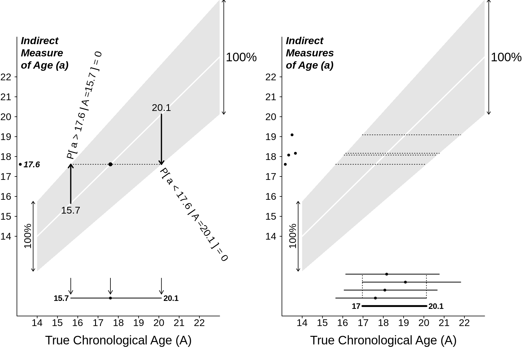
Figure 4.2: 100% Confidence Intervals for a person's chronological age when error distributions (that in this example are wider at the older ages) are 100% confined within the shaded ranges. Left: based on n = 1 measurement; right: based on n = 4 independent measurements.

More data

The panel on the right shows how, by obtaining 4 independent measurements, and finding the interval they have in common, you can narrow the interval containing the true age.

Can we narrow the interval more, maybe by first averaging the 4 measurements? Should the mean of 4 measurements give us more information, ie., a tighter interval, that the one based on the overlap? The sad fact is that, as long we insist on 100% confidence in our interval (or our procedure), we can not: the mean of the 3 measurements can still -- theoretically -- be anywhere in the same 0.75 \(\times\) True Age to 1.25 \(\times\) True Age range -- just as a single measurement can.

The only way to narrow the interval is to take a chance, cut corners, and accept a lower confidence level. To do this, we need to know a bit more about where the pattern (shape) of the error distribution (**up to now we didn't use the shape, just the boundaries). In other words, we need to know how much of the error distribution is in the corners, so that we can cut them!

In the next section, we will stick for now with Daniel Bernoulli's error distribution, but cut some corners. (Later on, we will cut some corners on Laplace's and Gauss's error distributions, but with the same standard deviation as in Bernoulli's error curve.)

4.2 More-nuanced intervals

We will cut 5% from each corner of the distribution, and focus on the middlemost 90%. From the formula for its mathematical shape, we can calculate that this measurement range is from -1 \(\times\) the radius of the semi-ellipse to +1 \(\times\) the radius. There is only a 5% probability of observing a measurement below (to the left of) this interval, and a 5% probability of observing a measurement above (to the right of) the interval. After we observe our single measurement, we 'try it on' against all possible true-age-scenarios. We retain only those true-age-scenarios in which the observed measurement would fall within this central (90%) range. We discard ('rule out') those age scenarios in which the measurement would be at one extreme or the other extreme, in one of the two excluded or 'cut' corners.

The left panel shows the (now narrower, and more nuanced) range of true-ages (rahe of parameter values) that is compatible with the observed measurement of 13.1 years. In all other age-scenarios, the 13.1 would have been too extreme, and so these scenarios are discarded. We can think of the 'ruled in' range as our (nuanced, compromise) parameter interval.

Note again the method of constructing this non-symmetric parameter interval, namely one boundary at a time. It does not fit the \(\pm\) mold.

It does, however, give a way of talk about such an interval:

The observed measurement (point-estimate) may be an underestimate of the parameter: it might have fallen short of the true parameter value. Or, it may be an underestimate: it might have overshot the true parameter value. The plus and the minus amounts are the almost-maximal amounts by which our shot might have been off-target. (as we will see later, the maximal error can be infinite, so we have to put some probalistic limits on the error if we are to narrow the interval).

Q: Does this procedure for constructing intervals have a 90% success rate, if used up and down all of the ages, say from 10 to 30 years? We could try it out with people of known ages. [answer by simulation]

You will discover in your simulations that it might matter whether you simulate the same number of 16 year olds as 10 years, i.e., what the mix of real ages is. This does not matter in the 100% intervals, but it might if you are more nuanced. For example,instead of estimating age by an indirect method, pretend you were were estimating a person's height indirectly, by just measuring their arm span (at each height, the mean armspan is very close to the height, but there is a spread of armspans (pardon the pun!)). And (just like in our example 2 where the spread increases with the mean) the spread of armspans is larger in people who are 6 feet tall than it is in people 5 feet tall. BUT, there aren't as many people 5 feet and 6 feet tall as there are people 5 feet 6 inches. So, the distribution of heights in people with a span of 5 feet 11 might have a different shape than that in people with a span of 5 feet 6, or 5 feet. Simulations (or even some diagrams) could settle the issue as to whether the height-mix (or, in example 2, the age mix) matters. What is your intuition as to whether it affects the perfornace of your nuanced parameter estimates? The point is that your method needs to have the same claimed performance (say 90%) at any age you throw at it.

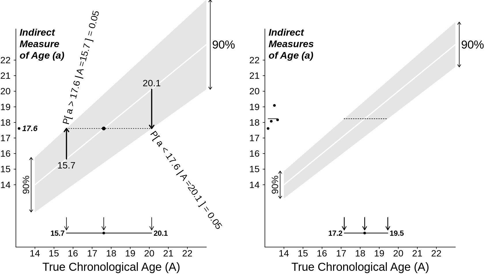
Figure 4.3: 90% Confidence intervals for Chronological Age when only 90% of the error distributions lie within the shaded ranges.

When we have \(n = 3\) observations (right panel), it is not so easy to say how confident we should be about the overlap of the 3 intervals. Instead, we would be bettter off taking the mean of the 3 measurements, and 'trying on' this single mean against the various sampling distributions of the means of 3 independent measurements from a semi-circular error distribution. Again, since the range remains the same, we would again have to cut corners. We will illustrate this when we now consider the easier-to-work-with Gaussian error distribution.

A more realistic error distribution

Although it makes it easier to demonstrate '100% confidence' intervals, Daniel Bernoulli's error distribution is both mathematically unfamiliar, and a bit unrealistic. And it isn't that easy to see how to use it for situations where you wiull want to take an average of several independent indirect measurements. So, we now switch to a more familiar and more realistic bell-shaped error distribution. It is often called the Gaussian distribution, even if Gauss was not the first to publish it. Variations of it were alraedy discovered by deMoivre many decades earlier, and Gauss' competotor, Laplace , publihed it well before Gauss did. Gauss claimed he was using it for many years before he published it. Laplace also used a different (more spiked) error distibution that today is called after him.

In any case, lets switch to bell-shaped distributions of the age measurements at each true age, but let's keep the 'average squared deviation' or its square root, the standard deviation, the same as it was in the Bernoulli model.

on 10 Mark note

NEXT

we deliberately took non-symmetric situations where it is not +/-

Now will show sitations where the error doesnt get bigger of smaller with the context, and where the 'trying-on' is faster.

4.3 SUMMARY

• what a parameter interval is

• If an error distribution is bounded, we can be 100% confident in our parameter interval, and we can narrow it by taking more measurements. Moreover, we don't need to specify the exact shape of the error distribution. All that matters are its bounds.

I don't think you should take for granted that students (or even professors!) will know what an error distribution is. So I think a first point should be to describe what you mean by an error distribution.

• With unbounded error distributions, a 100% parameter interval may be unacceptably wide, even if we take many measurements. Thus, we have to 'give up something' (in certainty) in order to 'get something' (a narrower interval). Moreover, we need to either (a) specify a model for the shape of the error distribution, or (b) use data-intensive techniques, such as re-sampling, to be able to 'cut the corners.'

• Either way, a logical way to determine parameter intervals is to have them consist of all the parameter-value scenarios in which the observed measurement (or summary measurement) is 'plausible'. The upper limit for the parameter is the scenario in which the measurement would be probalistically near the bottom of the corresponding sampling distribution; the lower limit is the scenario in which the measurement would be near the top of the corresponding sampling distribution.

• If the error (or sampling) distributions have differing spreads at different parameter values, then the parameter interval will not be symmetric about the point estimate. If the error (or sampling) distributions have the same spreads at different parameter values, then the parameter interval will be symmetric about the point estimate, and thus, easier to calculate.

it would be good to give a concrete example here.e.g. repeat the age example --> It's harder to accurately guess the true age of someone who is older. perhaps also a good time to mention that in this situation, the +/- formula will fail you

• It is not correct to view the parameter as 'falling' on one or other side of the measurement. The true parameter values is fixed, and isn't moving or falling anywhere. Rather, it is the observed measurement (point-estimate) that may have fallen to the left of (fallen short of), and thus provided an underestimate of, the true parameter value: Or, it may have overshot the true parameter value, and thus overestimated it.

This point also explains why the +/- formula fails us

Missing from the above summary points is a direct answer to the question or criticisms we are likely to face: "Why do we care about Wilson when the +/- gives you the same answer?" The answer to this question is given indirectly in points 4) and 5). But I think we need to be explicitly clear about this, since for me at least, is the main motivation for this chapter.

I also think the objective of the chapter needs to be revised. Based on our discussions, the point of the chapter is to explain: 1) Why the +/- formula fails us in the interpretation of a CI and when the spread of the error distribution is non-constant and 2) Wilson's idea to remedy the situation.

If you agree with those two objectives, the next question to answer is how '100% confidence intervals' and ultimately 'cutting corners' helps you explain the points 1) and 2).

By the way, a simplified version of the Wilson plot you made will be a great help in visualizing point 3:

---

Another unrealistic feature of our 'measurement model' is that the 'error distribution' has a semi-circular (or rather semi-eliptical) shape. In statistics, it is called the 'Wigner' semicircle distribution. First written about by Daniel Bernoulli, predates the error distributions of Laplace and Gauss.

5. If the archer makes innumerable shots, all with the utmost possible care, the arrows will strike sometimes the first band next to the mark, sometimes the second, sometimes the third and so on, and this is to be understood equally of either side whether left or right. Now is it not self-evident that the hits must be assumed to be thicker and more numerous on any given band the nearer this is to the mark? If all the places on the vertical plane, whatever their distance from the mark, were equally liable to be hit, the most skilful shot would have no advantage over a blind man. That, however, is the tacit assertion of those who use the common rule in estimating the value of various discrepant observations, when they treat them all indiscriminately. In this way, therefore, the degree of probability of any given deviation could be determined to some extent a posteriori, since there is no doubt that, for a large number of shots, the probability is proportional to the number of shots which hit a band situated at a given distance from the mark. Moreover, there is no doubt that the greatest deviation has its limits which are never exceeded and which indeed are narrowed by the experience and skill of the observer. Beyond these limits all probability is zero; from the limits towards the mark in the centre the probability increases and will be greatest at the mark itself. [Note: developers and teachers of statistical methods have long made use of archery, gunnery, darts, and aiming at targets. Indeed, the word stochastic, which refers to randomnees, has its roots in the Greek word stokhastikos, meaning able to guess, with the root stokhos meaning a target. Klein (1997) writes of 'men reasoning on the likes of target practice' and describes how this imagery has pervaded the thinking and work of natural philosophers and statisticians ]

6. The foregoing give some idea of a scale of probabilities for all deviations, such as each observer should form for himself. It will not be absolutely exact, but it will suit the nature of the inquiry well enough. The mark set up is, as it were, the centre of forces to which the observers are drawn; but these efforts are opposed by innumerable imperfections and other tiny hidden obstacles which may produce in the observations small chance errors. Some of these will be in the same direction and will be cumulative, others will cancel out, according as the observer is more or less lucky. From this it may be understood that there is some relation between the errors which occur and the actual true position of the centre of forces; for another position of the mark the outcome of chance would be estimated differently. So we arrive at the particular problem of determining the most probable position of the mark from a knowledge of the positions of some of the hits. It follows from what we have adduced that one should think above all of a scale (scala) between the various distances from the centre of forces and the corresponding probabilities. Vague as is the determination of this scale, it seems to be subject to various axioms which we have only to satisfy to be in a better case than if we suppose every deviation, whatever its magnitude, to occur with equal ease and therefore to have equal probability. Let us suppose a straight line in which there are disposed various points, which indicate of course the results of different observations. Let there be marked on this line some intermediate point which is taken as the true position to be determined. Let perpendiculars expressing the probability appropriate to a given point be erected. If now a curve is drawn through the ends of the several perpendiculars this will be the scale of the probabilities of which we are speaking.

7. If this is accepted, I think the following assumptions about the scale of probabilities can hardly be denied.

1. Inasmuch as deviations from the true intermediate point are equally easy in both directions, the scale will have two perfectly similar and equal branches.
2. Observations will certainly be more numerous and indeed more probable near to the centre of forces; at the same time they will be less numerous in proportion to their distance from that centre. The scale therefore on both sides approaches the straight line on which we supposed the observed points to be placed.
3. The degree of probability will be greatest in the middle where we suppose the centre of forces to be located, and the tangent to the scale for this point will be parallel to the aforesaid straight line.
4. If it is true, as I suppose, that even the least-favoured observations have their limits, best fixed by the observer himself, it follows that the scale, if correctly arranged, will meet the line of the observations at the limits themselves. For at both extremes all probability vanishes and a greater error is impossible.
5. Finally, the maximum deviations on either side are reckoned to be a sort of boundary between what can happen and what cannot. The last part, therefore, of the scale, on either side, should approach steeply the line on which the observations are sited, and the tangents at the extreme points will be almost perpendicular to that line. The scale itself will thus indicate that it is scarcely possible to pass beyond the supposed limits. Not that this condition should be applied in all its rigour if, that is, one does not fix the limits of error over-dogmatically.

8. If we now construct a semi-ellipse of any parameter on the line representing the whole field of possible deviations as its axis, this will certainly satisfy the foregoing conditions quite well. The parameter [radius] of the ellipse is arbitrary, since we are concerned only with the proportion between the probabilities of any given deviation. However elongated or com-pressed the ellipse may be, provided it is constructed on the same axis, it will perform the same function; which shows that we have no reason to be anxious about an accurate description of the scale. In fact we can even use a circle, not because it is proved to be the true scale by mathematical reasoning, but because it is nearer the truth than an infinite straight line parallel to the axis, which supposes that the several observations are of equal weight and probability, however distant from the true position. This circular scale also lends itself best to numerical calculations; meanwhile it is worth observing in advance that both hypotheses come to the same whenever the several observations are considered to be infinitely small. They also agree if the radius of the auxiliary circle is supposed to be infinitely large, as if no limits were set to the deviations. Thus if the deviation of an observation from the true position is thought of as the sine of a circular arc, the probability of that observation will be the cosine of the same arc. Let the auxiliary semicircle, which I have just described, be called the controlling semicircle (moderator). Where the centre of this semicircle is located, the true position, which fits the observations best, is to be fixed. Admittedly our hypothesis is, to some extent, precarious, but it is certainly to be preferred to the common one, and will not be hazardous to those who understand it, since the result that they will arrive at will always have a higher probability than if they had adhered to the common method. When by the nature of the case a certain decision cannot be reached, there is no other course than to prefer the more probable to the less probable.

9. I will illustrate this line of argument by a trivial example. The particular problem is the reconciliation of discrepant observations; it is therefore a question of difference of observations. Now if a dice-thrower makes three throws with one die so that the second exceeds the first by one and the third exceeds the second by two, the throws may arise in three ways, viz. 1,2,4 or 2,3,5 or 3,4,6. None of these throws is to be preferred to the other two, for each is in itself equally probable. If you prefer the one in the middle, viz. 2,3,5, the preference is illogical. The same sort of thing happens if you choose to consider observations which, so far as you are concerned, are accidental, whether they are astronomical or of some other kind, as equally probable. Now suppose the thrower produces the same result by throwing a pair of dice three times. There will then be eight different ways in which he would obtain this result, viz. 2,3,5; 3,4,6; 4,5,7; 5,6,8; 6,7,9; 7,8,10; 8,9,11 and 9,10,12. But they are far from being all equally probable. It is well known that the respective probabilities are proportional to the numbers 8, 30, 72, 100, 120, 80, 40 and 12. From this known scale I have better right to conclude that the fifth set has happened than that any other has, because it has the highest probability; and so the three throws of a pair of dice will have been 6, 7 and 9. No-one, however, will deny that the first set 2, 3 and 5 might possibly have happened, even though it has only a fifteenth part of the probability corresponding to the fifth set. Forced to choose, I simply choose what is most probable. Although this example does not quite square with our argument, it makes clear what contribution the investigation of probabilities can make to the determination of cases. Now I will come more to grips with the actual problem.

10. First of all, I would have every observer ponder thoroughly in his own mind and judge what is the greatest error which he is morally certain (though he should call down the wrath of heaven) he will never exceed however often he repeats the observation. He must be his own judge of his dexterity and not err on the side of severity or indulgence. Not that it matters very much whether the judgement he passes in this matter is fitting or somewhat flighty. Then let him make the radius of the controlling circle equal to the aforementioned greatest error; let this radius be r and hence the width of the whole doubtful field = 2r. If you desire a rule on this matter common to all observers, I recommend you to suit your judgement to the actual observations that you have made: if you double the distance between the two extreme observations, you can use it, I think, safely enough as the diameter of the controlling circle, or, what comes to the same thing, if you make the radius equal to the difference between the two extreme observations. Indeed, it will be sufficient to increase this difference by half to form the diameter of the circle if several observations have been made; my own practice is to double it for three or four observations, and .to increase it by half for more. Lest this uncertainty offend any one, it is as well to note that if we were to make our controlling semicircle infinite we should then coincide with the generally accepted rule of the arithmetical mean; but if we were to diminish the circle as much as possible without contradiction, we should obtain the mean between the two extreme observations, which as a rule for several observations I have found to be less often wrong than I thought before I investigated the matter.

We must wonder whether its was that this eminent mathematician (who also, incidentally contributed to the epidemiological debate about smallpox vaccination) was unable to think of a formula for an error distribution that did not end abruptly, and that would instead 'flow out' further in both directions. Or was it that he wasn't bothered by having to find the roots of 5th degree polynomials to find the best 'centre' of his semicircukar distribution? As it turns out, the mathematics involved in finding (what we now call today) the Maximun Likelihood Estimator for Laplace's and Gauss's (infinitely wide) error distributions is much simpler. But the, we have the benefit of hindsight.

The key ideas -- the semi-ellipse and the fixed (assumed known) -- are highlighted.